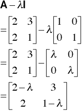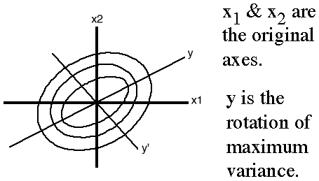
Consider

We wish to find V such that Σy2 is a maximum with the restriction that V'V = I.
Theorem 1
Given p variables which follow a p-variate normal distribution, the axis defining the linear transformation with maximum variance is the major axis of the isodensity hyperellipsoid

Σ is the covariance matrix, and C is an arbitrary positive constant.
Lagrange Multipliers
The method of Lagrange multipliers is convient. In this domain, the method is referred to as Eigenvalues and Eigenvectors. This method makes use of the formula,

in which λ is the eigenvalue and v is the eigenvector. The matrix of v's is used to define the transformation to maximum variance.
Synonyms
eigenvalue       characteristic root        latent root
eigenvector      characteristic vector      latent vector
Solution to Variance-Maximizing Rotations: Eigenvalue Problems
Consider the equation of the general form,  which translates to
 To solve for v, one must first find the value of λ.
Characteristic Equation
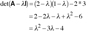
Eigenvalues found be solving the characteristic equation:
 If A is a 4x4 matrix then the solution to the characteristic equation will involve a 4th degree
polynomial and will yield up to four roots.
The Fundamental Theorem of Algebra
Every polynomial of degree n, where n is greater than or equal to one, with real
or complex coefficients has n real or complex roots.
Gauss, 1797
Characteristic Vectors v
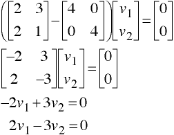
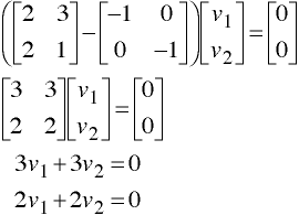
Eigenvectors are found using λ and solving for v.

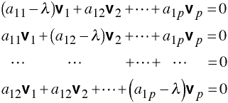
Solving for v involves solving a system of p simultaneous equations in p unknowns, such as:
Rotation for Maximum Variance
The eignevectors are used to describe the orthogonal rotation from maximum variance. This type of rotation is often referred to as principal-axes rotation.
Properties of Matrices Related to Eigenvalues and Eigenvectors
Theorem 2
The sum Σλi of the eigenvlaues of a matrix A is equal to the trace of A, tr(A).
Theorem 3
The product of the λi,
 of the eigenvlaues of a matrix
A is equal to the determinant of A, Det(A).
Theorem 4
Two eigenvectors vi and vj associated with two distinct eigenvalues λi and λj of a symmetric matrix are mutually orthogonal, v'ivj = 0.
Theorem 5
Given a set of variables X1, X2, ...,Xp, with nonsingular covariance matrix Σ, we can always derive a set of uncorrelated variables Y1, Y2, ..., Yp by a set of linear transforamtions corresponding to the principal-axes rotation. The covariance matrix of this new set of variables is the diagonal matrix Λ = V'ΣV
Theorem 6
Given a set of variables X1, X2, ...,Xp, with nonsingular covariance matrix Σx, a new set of variables Y1, Y2, ..., Yp is defined by the transformation Y' = X'V, where V is an orthogonal matrix. If the covariance matrix of the Y's is Σy, then the following relation holds:
 In other words, the quadratic form is invariant under rigid rotation.
Definition


