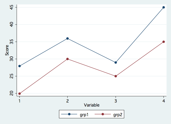
Consider the graph below which shows the profiles for two groups. The question that we try to answer in profile analysis is whether or not the profiles are equivalent, i.e., are the profiles piecewise parallel. Then, if it is true that the profiles are parallel, are there group differences, i.e., is the separation of the profiles significant. Finally, if it is true that the profiles are parallel, are the profiles flat, i.e., are values of the dependent variables the same. Please note that when doing profile analysis you need the different dependent variables to be commensurable, i.e., expressed in comparable units.
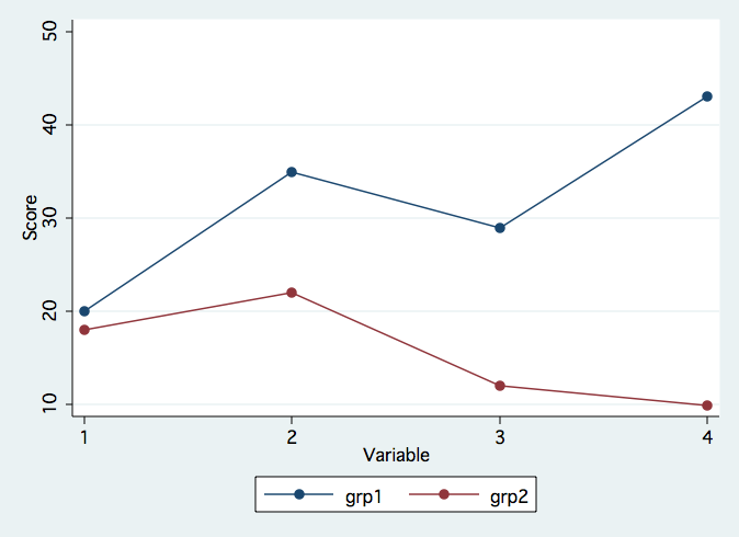
Contrast the graph above with the one below in which the profiles are clearly not the same.
Profile analysis is really just a kind of repeated measures mixed models analysis. There are some tricks to doing the analysis such that we can test the piecewise parallelness. Here is a summary of the various test that are performed in a profile analysis.
We begin by testing for parallelism. If the profiles are not piecewise parallel then the remaining tests do not make a whole lot of sense.
We begin with a standard one-way manova followed by a test that use a transformation of the dependent variables defined by the transformation matrix c1.
                    1  -1   0   0
             c1  =  0   1  -1   0
                    0   0   1  -1
This is actually a group by DV interaction.2. Test of Levels (Group differences)
If we have parallelism than we can test whether there is a difference in the groups. We do this with another transformation matrix, c2.
c1 = 1 1 1 1This tests for groups differences by summing across the dependent variables.
3. Test of Flatness
Lastly, we can test whether the profiles are flat by using the c1 transformation against the intercept term. By using different transformations of the dependent variables we can test hypotheses about trend across the dependent variables. Here are the transformation matrices using coefficients for orthogonal polynomials for linear (o1) and nonlinear (o2) effects.
                  o1  =  -3  -1   1   3


                  o2  =   1  -1  -1   1
                         -1   3  -3   1
Here is an example of a simple profile analysis with four groups and three dependent variables.
input id y1 y2 y3 grp
1 19 20 18 1
2 20 21 19 1
3 19 22 22 1
4 18 19 21 1
5 16 18 20 1
6 17 22 19 1
7 20 19 20 1
8 15 19 19 1
9 12 14 12 2
10 15 15 17 2
11 15 17 15 2
12 13 14 14 2
13 14 16 13 2
14 15 14 17 3
15 13 14 15 3
16 12 15 15 3
17 12 13 13 3
18 8 9 10 4
19 10 10 12 4
20 11 10 10 4
21 11 7 12 4
end
tabstat y1 y2 y3, by(grp)
Summary statistics: mean
by categories of: grp
grp | y1 y2 y3
---------+------------------------------
1 | 18 20 19.75
2 | 13.8 15.2 14.2
3 | 13 14 15
4 | 10 9 11
---------+------------------------------
Total | 14.52381 15.61905 15.85714
----------------------------------------
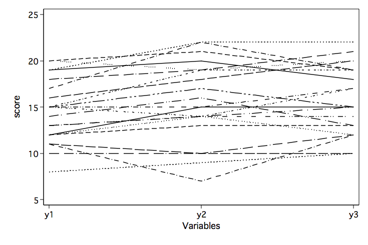
/* profile plot by individual -- findit profileplot */
profileplot y1 y2 y3, by(id) legend(off) nosymbols ytitle(score)
 /* preliminary one-way manova */
manova y1 y2 y3 = grp
Number of obs = 21
W = Wilks' lambda L = Lawley-Hotelling trace
P = Pillai's trace R = Roy's largest root
Source | Statistic df F(df1, df2) = F Prob>F
-----------+--------------------------------------------------
grp | W 0.0479 3 9.0 36.7 10.12 0.0000 a
| P 1.1609 9.0 51.0 3.58 0.0016 a
| L 15.6417 9.0 41.0 23.75 0.0000 a
| R 15.3753 3.0 17.0 87.13 0.0000 u
|--------------------------------------------------
Residual | 17
-----------+--------------------------------------------------
Total | 20
--------------------------------------------------------------
e = exact, a = approximate, u = upper bound on F
/* test of parallelism */
mat c1 = (1,-1,0\0,1,-1)
manovatest grp, ytrans(c1)
Transformations of the dependent variables
(1) y1 - y2
(2) y2 - y3
W = Wilks' lambda L = Lawley-Hotelling trace
P = Pillai's trace R = Roy's largest root
Source | Statistic df F(df1, df2) = F Prob>F
-----------+--------------------------------------------------
grp | W 0.5633 3 6.0 32.0 1.77 0.1364 e
| P 0.4873 6.0 34.0 1.83 0.1234 a
| L 0.6853 6.0 30.0 1.71 0.1522 a
| R 0.5088 3.0 17.0 2.88 0.0662 u
|--------------------------------------------------
Residual | 17
--------------------------------------------------------------
e = exact, a = approximate, u = upper bound on F
/* test of levels */
mat c2 = (1,1,1)
manovatest grp, ytrans(c2)
Transformation of the dependent variables
(1) y1 + y2 + y3
W = Wilks' lambda L = Lawley-Hotelling trace
P = Pillai's trace R = Roy's largest root
Source | Statistic df F(df1, df2) = F Prob>F
-----------+--------------------------------------------------
grp | W 0.0740 3 3.0 17.0 70.93 0.0000 e
| P 0.9260 3.0 17.0 70.93 0.0000 e
| L 12.5165 3.0 17.0 70.93 0.0000 e
| R 12.5165 3.0 17.0 70.93 0.0000 e
|--------------------------------------------------
Residual | 17
--------------------------------------------------------------
e = exact, a = approximate, u = upper bound on
/* test of flatness */
mat xm = (1,0,0,0,0) /* used to select the constant only */
manovatest, test(xm) ytrans(c1)
Transformations of the dependent variables
(1) y1 - y2
(2) y2 - y3
Test constraint
(1) _cons = 0
W = Wilks' lambda L = Lawley-Hotelling trace
P = Pillai's trace R = Roy's largest root
Source | Statistic df F(df1, df2) = F Prob>F
-----------+--------------------------------------------------
manovatest | W 0.7927 1 2.0 16.0 2.09 0.1559 e
| P 0.2073 2.0 16.0 2.09 0.1559 e
| L 0.2615 2.0 16.0 2.09 0.1559 e
| R 0.2615 2.0 16.0 2.09 0.1559 e
|--------------------------------------------------
Residual | 17
--------------------------------------------------------------
e = exact, a = approximate, u = upper bound on F
/* orthogonal polynomials */
/* linear */
mat o1 = (-1,0,1)
manovatest grp, ytrans(o1)
Transformation of the dependent variables
(1) - y1 + y3
W = Wilks' lambda L = Lawley-Hotelling trace
P = Pillai's trace R = Roy's largest root
Source | Statistic df F(df1, df2) = F Prob>F
-----------+--------------------------------------------------
grp | W 0.8487 3 3.0 17.0 1.01 0.4126 e
| P 0.1513 3.0 17.0 1.01 0.4126 e
| L 0.1782 3.0 17.0 1.01 0.4126 e
| R 0.1782 3.0 17.0 1.01 0.4126 e
|--------------------------------------------------
Residual | 17
--------------------------------------------------------------
e = exact, a = approximate, u = upper bound on F
/* quadratic */
mat o2 = (1,-2,1)
manovatest grp, ytrans(o2)
Transformation of the dependent variables
(1) y1 - 2 y2 + y3
W = Wilks' lambda L = Lawley-Hotelling trace
P = Pillai's trace R = Roy's largest root
Source | Statistic df F(df1, df2) = F Prob>F
-----------+--------------------------------------------------
grp | W 0.6678 3 3.0 17.0 2.82 0.0702 e
| P 0.3322 3.0 17.0 2.82 0.0702 e
| L 0.4974 3.0 17.0 2.82 0.0702 e
| R 0.4974 3.0 17.0 2.82 0.0702 e
|--------------------------------------------------
Residual | 17
--------------------------------------------------------------
e = exact, a = approximate, u = upper bound on F
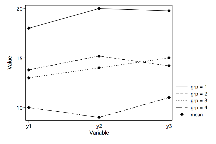
/* profile plot by groups -- findit profileplot */
profileplot y1 y2 y3, by(grp) xtitle(Variable) ytitle(Value)
/* preliminary one-way manova */
manova y1 y2 y3 = grp
Number of obs = 21
W = Wilks' lambda L = Lawley-Hotelling trace
P = Pillai's trace R = Roy's largest root
Source | Statistic df F(df1, df2) = F Prob>F
-----------+--------------------------------------------------
grp | W 0.0479 3 9.0 36.7 10.12 0.0000 a
| P 1.1609 9.0 51.0 3.58 0.0016 a
| L 15.6417 9.0 41.0 23.75 0.0000 a
| R 15.3753 3.0 17.0 87.13 0.0000 u
|--------------------------------------------------
Residual | 17
-----------+--------------------------------------------------
Total | 20
--------------------------------------------------------------
e = exact, a = approximate, u = upper bound on F
/* test of parallelism */
mat c1 = (1,-1,0\0,1,-1)
manovatest grp, ytrans(c1)
Transformations of the dependent variables
(1) y1 - y2
(2) y2 - y3
W = Wilks' lambda L = Lawley-Hotelling trace
P = Pillai's trace R = Roy's largest root
Source | Statistic df F(df1, df2) = F Prob>F
-----------+--------------------------------------------------
grp | W 0.5633 3 6.0 32.0 1.77 0.1364 e
| P 0.4873 6.0 34.0 1.83 0.1234 a
| L 0.6853 6.0 30.0 1.71 0.1522 a
| R 0.5088 3.0 17.0 2.88 0.0662 u
|--------------------------------------------------
Residual | 17
--------------------------------------------------------------
e = exact, a = approximate, u = upper bound on F
/* test of levels */
mat c2 = (1,1,1)
manovatest grp, ytrans(c2)
Transformation of the dependent variables
(1) y1 + y2 + y3
W = Wilks' lambda L = Lawley-Hotelling trace
P = Pillai's trace R = Roy's largest root
Source | Statistic df F(df1, df2) = F Prob>F
-----------+--------------------------------------------------
grp | W 0.0740 3 3.0 17.0 70.93 0.0000 e
| P 0.9260 3.0 17.0 70.93 0.0000 e
| L 12.5165 3.0 17.0 70.93 0.0000 e
| R 12.5165 3.0 17.0 70.93 0.0000 e
|--------------------------------------------------
Residual | 17
--------------------------------------------------------------
e = exact, a = approximate, u = upper bound on
/* test of flatness */
mat xm = (1,0,0,0,0) /* used to select the constant only */
manovatest, test(xm) ytrans(c1)
Transformations of the dependent variables
(1) y1 - y2
(2) y2 - y3
Test constraint
(1) _cons = 0
W = Wilks' lambda L = Lawley-Hotelling trace
P = Pillai's trace R = Roy's largest root
Source | Statistic df F(df1, df2) = F Prob>F
-----------+--------------------------------------------------
manovatest | W 0.7927 1 2.0 16.0 2.09 0.1559 e
| P 0.2073 2.0 16.0 2.09 0.1559 e
| L 0.2615 2.0 16.0 2.09 0.1559 e
| R 0.2615 2.0 16.0 2.09 0.1559 e
|--------------------------------------------------
Residual | 17
--------------------------------------------------------------
e = exact, a = approximate, u = upper bound on F
/* orthogonal polynomials */
/* linear */
mat o1 = (-1,0,1)
manovatest grp, ytrans(o1)
Transformation of the dependent variables
(1) - y1 + y3
W = Wilks' lambda L = Lawley-Hotelling trace
P = Pillai's trace R = Roy's largest root
Source | Statistic df F(df1, df2) = F Prob>F
-----------+--------------------------------------------------
grp | W 0.8487 3 3.0 17.0 1.01 0.4126 e
| P 0.1513 3.0 17.0 1.01 0.4126 e
| L 0.1782 3.0 17.0 1.01 0.4126 e
| R 0.1782 3.0 17.0 1.01 0.4126 e
|--------------------------------------------------
Residual | 17
--------------------------------------------------------------
e = exact, a = approximate, u = upper bound on F
/* quadratic */
mat o2 = (1,-2,1)
manovatest grp, ytrans(o2)
Transformation of the dependent variables
(1) y1 - 2 y2 + y3
W = Wilks' lambda L = Lawley-Hotelling trace
P = Pillai's trace R = Roy's largest root
Source | Statistic df F(df1, df2) = F Prob>F
-----------+--------------------------------------------------
grp | W 0.6678 3 3.0 17.0 2.82 0.0702 e
| P 0.3322 3.0 17.0 2.82 0.0702 e
| L 0.4974 3.0 17.0 2.82 0.0702 e
| R 0.4974 3.0 17.0 2.82 0.0702 e
|--------------------------------------------------
Residual | 17
--------------------------------------------------------------
e = exact, a = approximate, u = upper bound on F
/* profile plot by groups -- findit profileplot */
profileplot y1 y2 y3, by(grp) xtitle(Variable) ytitle(Value)
use hsb2, clear

/* preliminary one-way manova */
manova read write math science socst = prog

                           Number of obs =     200

                           W = Wilks' lambda      L = Lawley-Hotelling trace
                           P = Pillai's trace     R = Roy's largest root

                  Source |  Statistic     df   F(df1,    df2) =   F   Prob>F
              -----------+--------------------------------------------------
                    prog | W   0.6682      2    10.0   386.0     8.62 0.0000 e
                         | P   0.3413           10.0   388.0     7.98 0.0000 a
                         | L   0.4826           10.0   384.0     9.27 0.0000 a
                         | R   0.4514            5.0   194.0    17.51 0.0000 u
                         |--------------------------------------------------
                Residual |               197
              -----------+--------------------------------------------------
                   Total |               199
              --------------------------------------------------------------
                           e = exact, a = approximate, u = upper bound on F

/* test of parallelism */
mat c1 = (1,-1,0,0,0\0,1,-1,0,0\0,0,1,-1,0\0,0,0,1,-1)

manovatest prog, ytrans(c1)

 Transformations of the dependent variables
 (1)    read - write
 (2)    write - math
 (3)    math - science
 (4)    science - socst

                           W = Wilks' lambda      L = Lawley-Hotelling trace
                           P = Pillai's trace     R = Roy's largest root

                  Source |  Statistic     df   F(df1,    df2) =   F   Prob>F
              -----------+--------------------------------------------------
                    prog | W   0.8983      2     8.0   388.0     2.67 0.0072 e
                         | P   0.1025            8.0   390.0     2.63 0.0081 a
                         | L   0.1125            8.0   386.0     2.71 0.0064 a
                         | R   0.1047            4.0   195.0     5.10 0.0006 u
                         |--------------------------------------------------
                Residual |               197
              --------------------------------------------------------------
                           e = exact, a = approximate, u = upper bound on F

/* profile plot -- findit profileplot */

profileplot read write math science socst, by(prog) xtitle(Variable) ytitle(Mean Score)
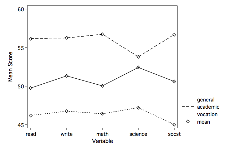
The lack of parallelism is most likely because the top line goes down and then up for the last
two variables while in the bottom two lines the pattern is up then down.
use http://www.philender.com/courses/data/deprofile, clear
tabstat dep1 dep2 dep3 dep4, by(group)
Summary statistics: mean
by categories of: group
group | dep1 dep2 dep3 dep4
---------+----------------------------------------
placebo | 16.58824 14.97294 14.12882 12.27471
estrogen | 12.9825 11.17286 8.924643 8.827857
---------+----------------------------------------
Total | 14.34467 12.60844 10.89067 10.13
--------------------------------------------------
/* profile plot by individual */
reshape long dep, i(subj) j(v)
(note: j = 1 2 3 4)
Data wide -> long
-----------------------------------------------------------------------------
Number of obs. 45 -> 180
Number of variables 6 -> 4
j variable (4 values) -> v
xij variables:
dep1 dep2 ... dep4 -> dep
-----------------------------------------------------------------------------
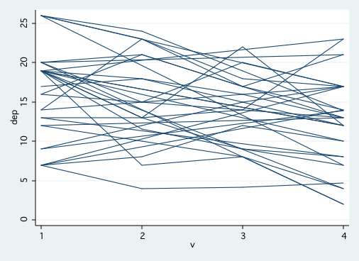
/* placebo group */
twoway line dep v if group==0
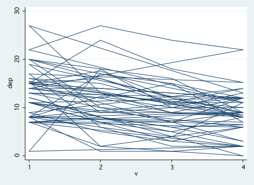
 /* estrogen group */
twoway line dep v if group==1
/* estrogen group */
twoway line dep v if group==1
 reshape wide
(note: j = 1 2 3 4)
Data long -> wide
-----------------------------------------------------------------------------
Number of obs. 180 -> 45
Number of variables 4 -> 6
j variable (4 values) v -> (dropped)
xij variables:
dep -> dep1 dep2 ... dep4
-----------------------------------------------------------------------------
/* preliminary one-way manova */
manova dep1 dep2 dep3 dep4 = group
Number of obs = 45
W = Wilks' lambda L = Lawley-Hotelling trace
P = Pillai's trace R = Roy's largest root
Source | Statistic df F(df1, df2) = F Prob>F
-----------+--------------------------------------------------
group | W 0.7623 1 4.0 40.0 3.12 0.0253 e
| P 0.2377 4.0 40.0 3.12 0.0253 e
| L 0.3117 4.0 40.0 3.12 0.0253 e
| R 0.3117 4.0 40.0 3.12 0.0253 e
|--------------------------------------------------
Residual | 43
-----------+--------------------------------------------------
Total | 44
--------------------------------------------------------------
e = exact, a = approximate, u = upper bound on F
/* test of parallelism */
mat c1 = (1,-1,0,0\0,1,-1,0\0,0,1,-1)
manovatest group, ytrans(c1)
Transformations of the dependent variables
(1) dep1 - dep2
(2) dep2 - dep3
(3) dep3 - dep4
W = Wilks' lambda L = Lawley-Hotelling trace
P = Pillai's trace R = Roy's largest root
Source | Statistic df F(df1, df2) = F Prob>F
-----------+--------------------------------------------------
group | W 0.9095 1 3.0 41.0 1.36 0.2684 e
| P 0.0905 3.0 41.0 1.36 0.2684 e
| L 0.0995 3.0 41.0 1.36 0.2684 e
| R 0.0995 3.0 41.0 1.36 0.2684 e
|--------------------------------------------------
Residual | 43
--------------------------------------------------------------
e = exact, a = approximate, u = upper bound on F
/* test of levels */
mat c2 = (1,1,1,1)
manovatest group, ytrans(c2)
Transformation of the dependent variables
(1) dep1 + dep2 + dep3 + dep4
W = Wilks' lambda L = Lawley-Hotelling trace
P = Pillai's trace R = Roy's largest root
Source | Statistic df F(df1, df2) = F Prob>F
-----------+--------------------------------------------------
group | W 0.8448 1 1.0 43.0 7.90 0.0074 e
| P 0.1552 1.0 43.0 7.90 0.0074 e
| L 0.1837 1.0 43.0 7.90 0.0074 e
| R 0.1837 1.0 43.0 7.90 0.0074 e
|--------------------------------------------------
Residual | 43
--------------------------------------------------------------
e = exact, a = approximate, u = upper bound on F
/* test of flatness */
mat xm = (1,0,0) /* used to select the constant only */
manovatest, test(xm) ytrans(c1)
Transformations of the dependent variables
(1) dep1 - dep2
(2) dep2 - dep3
(3) dep3 - dep4
Test constraint
(1) _cons = 0
W = Wilks' lambda L = Lawley-Hotelling trace
P = Pillai's trace R = Roy's largest root
Source | Statistic df F(df1, df2) = F Prob>F
-----------+--------------------------------------------------
manovatest | W 0.6104 1 3.0 41.0 8.72 0.0001 e
| P 0.3896 3.0 41.0 8.72 0.0001 e
| L 0.6383 3.0 41.0 8.72 0.0001 e
| R 0.6383 3.0 41.0 8.72 0.0001 e
|--------------------------------------------------
Residual | 43
--------------------------------------------------------------
e = exact, a = approximate, u = upper bound on F
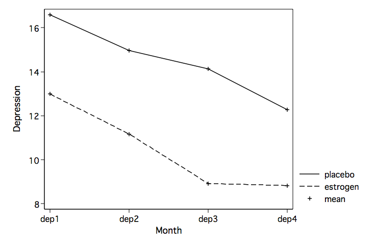
/* profile plot by groups */
tabstat dep1 dep2 dep3 dep4, by(group)
Summary statistics: mean
by categories of: group
group | dep1 dep2 dep3 dep4
---------+----------------------------------------
placebo | 16.58824 14.97294 14.12882 12.27471
estrogen | 12.9825 11.17286 8.924643 8.827857
---------+----------------------------------------
Total | 14.34467 12.60844 10.89067 10.13
--------------------------------------------------
/* findit profileplot */
profileplot dep1 dep2 dep3 dep4, by(group) xtitle(Month) ytitle(Depression)
reshape wide
(note: j = 1 2 3 4)
Data long -> wide
-----------------------------------------------------------------------------
Number of obs. 180 -> 45
Number of variables 4 -> 6
j variable (4 values) v -> (dropped)
xij variables:
dep -> dep1 dep2 ... dep4
-----------------------------------------------------------------------------
/* preliminary one-way manova */
manova dep1 dep2 dep3 dep4 = group
Number of obs = 45
W = Wilks' lambda L = Lawley-Hotelling trace
P = Pillai's trace R = Roy's largest root
Source | Statistic df F(df1, df2) = F Prob>F
-----------+--------------------------------------------------
group | W 0.7623 1 4.0 40.0 3.12 0.0253 e
| P 0.2377 4.0 40.0 3.12 0.0253 e
| L 0.3117 4.0 40.0 3.12 0.0253 e
| R 0.3117 4.0 40.0 3.12 0.0253 e
|--------------------------------------------------
Residual | 43
-----------+--------------------------------------------------
Total | 44
--------------------------------------------------------------
e = exact, a = approximate, u = upper bound on F
/* test of parallelism */
mat c1 = (1,-1,0,0\0,1,-1,0\0,0,1,-1)
manovatest group, ytrans(c1)
Transformations of the dependent variables
(1) dep1 - dep2
(2) dep2 - dep3
(3) dep3 - dep4
W = Wilks' lambda L = Lawley-Hotelling trace
P = Pillai's trace R = Roy's largest root
Source | Statistic df F(df1, df2) = F Prob>F
-----------+--------------------------------------------------
group | W 0.9095 1 3.0 41.0 1.36 0.2684 e
| P 0.0905 3.0 41.0 1.36 0.2684 e
| L 0.0995 3.0 41.0 1.36 0.2684 e
| R 0.0995 3.0 41.0 1.36 0.2684 e
|--------------------------------------------------
Residual | 43
--------------------------------------------------------------
e = exact, a = approximate, u = upper bound on F
/* test of levels */
mat c2 = (1,1,1,1)
manovatest group, ytrans(c2)
Transformation of the dependent variables
(1) dep1 + dep2 + dep3 + dep4
W = Wilks' lambda L = Lawley-Hotelling trace
P = Pillai's trace R = Roy's largest root
Source | Statistic df F(df1, df2) = F Prob>F
-----------+--------------------------------------------------
group | W 0.8448 1 1.0 43.0 7.90 0.0074 e
| P 0.1552 1.0 43.0 7.90 0.0074 e
| L 0.1837 1.0 43.0 7.90 0.0074 e
| R 0.1837 1.0 43.0 7.90 0.0074 e
|--------------------------------------------------
Residual | 43
--------------------------------------------------------------
e = exact, a = approximate, u = upper bound on F
/* test of flatness */
mat xm = (1,0,0) /* used to select the constant only */
manovatest, test(xm) ytrans(c1)
Transformations of the dependent variables
(1) dep1 - dep2
(2) dep2 - dep3
(3) dep3 - dep4
Test constraint
(1) _cons = 0
W = Wilks' lambda L = Lawley-Hotelling trace
P = Pillai's trace R = Roy's largest root
Source | Statistic df F(df1, df2) = F Prob>F
-----------+--------------------------------------------------
manovatest | W 0.6104 1 3.0 41.0 8.72 0.0001 e
| P 0.3896 3.0 41.0 8.72 0.0001 e
| L 0.6383 3.0 41.0 8.72 0.0001 e
| R 0.6383 3.0 41.0 8.72 0.0001 e
|--------------------------------------------------
Residual | 43
--------------------------------------------------------------
e = exact, a = approximate, u = upper bound on F
/* profile plot by groups */
tabstat dep1 dep2 dep3 dep4, by(group)
Summary statistics: mean
by categories of: group
group | dep1 dep2 dep3 dep4
---------+----------------------------------------
placebo | 16.58824 14.97294 14.12882 12.27471
estrogen | 12.9825 11.17286 8.924643 8.827857
---------+----------------------------------------
Total | 14.34467 12.60844 10.89067 10.13
--------------------------------------------------
/* findit profileplot */
profileplot dep1 dep2 dep3 dep4, by(group) xtitle(Month) ytitle(Depression)
Multivariate Course Page
Phil Ender, 1nov07, 3dec04