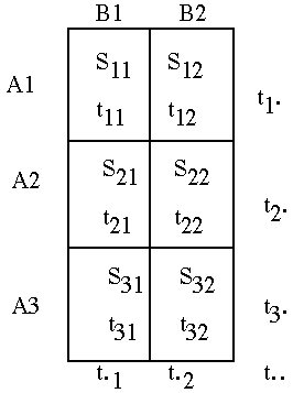
Consider the Design
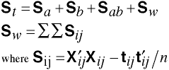
SSCP Matrices
Tests of Significance
Wilks' Lambda
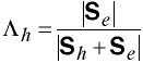
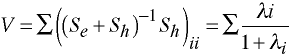
where Se represents the error SSCP matrix and Sh represents the hypothesis SSCP matrix.
For Example
In a fixed effects model, Sw is the Se for all effects.
While in the randoms effects model Sab is the Se for the main effects and Sw for the interaction.
If A is fixed and B is random th Sab is the Se for A main effect and Sw is the Se for the B main effect and the interaction.
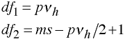
Rao's F Approximation
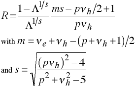
Degreees of Freedom
Special Note Concerning s
If either the numerator or the deminator of s equals 0 set s = 1.
Other Test Criteria
Hotelling's Trace Criterion
![]()
Roy's Largest Latent Root
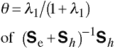
Pillai's Trace Criterion
Which of these is "best?"
Stata Manova Example
use http://www.gseis.ucla.edu/courses/data/hsb2

table prog female, cont(freq mean read mean write mean math)

------------------------------
type of   |       female
program   |     male    female
----------+-------------------
  general |       21        24
          | 52.95238  46.95833
          | 49.14286     53.25
          | 50.19048    49.875
          |
 academic |       47        58
          |  56.2766  56.06897
          | 54.61702  57.58621
          | 57.12766  56.41379
          |
 vocation |       23        27
          | 45.65217  46.66667
          | 41.82609  50.96296
          | 46.91304        46
------------------------------

corr read write math
(obs=200)

             |     read    write     math
-------------+---------------------------
        read |   1.0000
       write |   0.5968   1.0000
        math |   0.6623   0.6174   1.0000

manova read write math = prog female prog*female

                           Number of obs =     200

                           W = Wilks' lambda      L = Lawley-Hotelling trace
                           P = Pillai's trace     R = Roy's largest root

                  Source |  Statistic     df   F(df1,    df2) =   F   Prob>F
             ------------+--------------------------------------------------
                   Model | W   0.5808      5    15.0   530.4     7.69 0.0000 a
                         | P   0.4796           15.0   582.0     7.38 0.0000 a
                         | L   0.6206           15.0   572.0     7.89 0.0000 a
                         | R   0.3762            5.0   194.0    14.59 0.0000 u
                         |--------------------------------------------------
                Residual |               194
             ------------+--------------------------------------------------
                    prog | W   0.7305      2     6.0   384.0    10.88 0.0000 e
                         | P   0.2712            6.0   386.0    10.09 0.0000 a
                         | L   0.3666            6.0   382.0    11.67 0.0000 a
                         | R   0.3602            3.0   193.0    23.17 0.0000 u
                         |--------------------------------------------------
                  female | W   0.8238      1     3.0   192.0    13.69 0.0000 e
                         | P   0.1762            3.0   192.0    13.69 0.0000 e
                         | L   0.2139            3.0   192.0    13.69 0.0000 e
                         | R   0.2139            3.0   192.0    13.69 0.0000 e
                         |--------------------------------------------------
             prog*female | W   0.9321      2     6.0   384.0     2.29 0.0347 e
                         | P   0.0691            6.0   386.0     2.30 0.0338 a
                         | L   0.0716            6.0   382.0     2.28 0.0356 a
                         | R   0.0381            3.0   193.0     2.45 0.0646 u
                         |--------------------------------------------------
                Residual |               194
             ------------+--------------------------------------------------
                   Total |               199
             ---------------------------------------------------------------
                           e = exact, a = approximate, u = upper bound on F
We can look at the simultaneous confidence intervals for all pairwise combinations
of the means by converting the 3x2 design into a one-way design with six levels. We
can then use the Heck Charts with s=3, m=.5, n=95 and cv=.095.
egen grp = group(prog female)

tablist grp prog female, sort(v) nolabel clean    /* findit tablist */

    grp   prog   female   Freq
      1      1        0     21
      2      1        1     24
      3      2        0     47
      4      2        1     58
      5      3        0     23
      6      3        1     27

 manova read write math = grp

                           Number of obs =     200

                           W = Wilks' lambda      L = Lawley-Hotelling trace
                           P = Pillai's trace     R = Roy's largest root

                  Source |  Statistic     df   F(df1,    df2) =   F   Prob>F
              -----------+--------------------------------------------------
                     grp | W   0.5808      5    15.0   530.4     7.69 0.0000 a
                         | P   0.4796           15.0   582.0     7.38 0.0000 a
                         | L   0.6206           15.0   572.0     7.89 0.0000 a
                         | R   0.3762            5.0   194.0    14.59 0.0000 u
                         |--------------------------------------------------
                Residual |               194
              -----------+--------------------------------------------------
                   Total |               199
              --------------------------------------------------------------
                           e = exact, a = approximate, u = upper bound on F

manovatest, showorder

 Order of columns in the design matrix
      1: _cons
      2: (grp==1)
      3: (grp==2)
      4: (grp==3)
      5: (grp==4)
      6: (grp==5)
      7: (grp==6)

simulci read write math, by(grp) cv(.095)

s=3  m=.5  n=95 cv= .095

group variable:   grp

                                    pairwise simultaneous
comparison           difference      confidence intervals
dv: read
grp 1 vs grp 2        5.994        -2.401        14.390
grp 1 vs grp 3       -3.324       -11.720         5.071
grp 1 vs grp 4       -3.117       -11.512         5.279
grp 1 vs grp 5        7.300        -1.095        15.696
grp 1 vs grp 6        6.286        -2.110        14.681
grp 2 vs grp 3       -9.318*      -17.714        -0.923
grp 2 vs grp 4       -9.111*      -17.506        -0.715
grp 2 vs grp 5        1.306        -7.089         9.702
grp 2 vs grp 6        0.292        -8.104         8.687
grp 3 vs grp 4        0.208        -8.188         8.603
grp 3 vs grp 5       10.624*        2.229        19.020
grp 3 vs grp 6        9.610*        1.214        18.005
grp 4 vs grp 5       10.417*        2.021        18.812
grp 4 vs grp 6        9.402*        1.007        17.798
grp 5 vs grp 6       -1.014        -9.410         7.381

dv: write
grp 1 vs grp 2       -4.107       -11.566         3.351
grp 1 vs grp 3       -5.474       -12.933         1.984
grp 1 vs grp 4       -8.443*      -15.902        -0.985
grp 1 vs grp 5        7.317        -0.142        14.775
grp 1 vs grp 6       -1.820        -9.279         5.638
grp 2 vs grp 3       -1.367        -8.826         6.091
grp 2 vs grp 4       -4.336       -11.795         3.122
grp 2 vs grp 5       11.424*        3.965        18.882
grp 2 vs grp 6        2.287        -5.171         9.746
grp 3 vs grp 4       -2.969       -10.428         4.489
grp 3 vs grp 5       12.791*        5.332        20.249
grp 3 vs grp 6        3.654        -3.804        11.113
grp 4 vs grp 5       15.760*        8.302        23.219
grp 4 vs grp 6        6.623        -0.835        14.082
grp 5 vs grp 6       -9.137*      -16.595        -1.678

dv: math
grp 1 vs grp 2        0.315        -7.196         7.827
grp 1 vs grp 3       -6.937       -14.449         0.575
grp 1 vs grp 4       -6.223       -13.735         1.289
grp 1 vs grp 5        3.277        -4.234        10.789
grp 1 vs grp 6        4.190        -3.321        11.702
grp 2 vs grp 3       -7.253       -14.765         0.259
grp 2 vs grp 4       -6.539       -14.051         0.973
grp 2 vs grp 5        2.962        -4.550        10.474
grp 2 vs grp 6        3.875        -3.637        11.387
grp 3 vs grp 4        0.714        -6.798         8.226
grp 3 vs grp 5       10.215*        2.703        17.727
grp 3 vs grp 6       11.128*        3.616        18.640
grp 4 vs grp 5        9.501*        1.989        17.013
grp 4 vs grp 6       10.414*        2.902        17.926
grp 5 vs grp 6        0.913        -6.599         8.425
Even though Stata has a general purpose manova command that can do factorial designs. We will
demonstrate the use of mvreg (multivariate regression) along with the mvtest
command by David E. Moore of the University of Cincinnati (findit mvtest).
xi3: mvreg read write math = r.female*r.prog
r.female          _Ifemale_0-1        (naturally coded; _Ifemale_0 omitted)
r.prog            _Iprog_1-3          (naturally coded; _Iprog_1 omitted)
r.fem~e*r.prog    _IfemXpro_#_#       (coded as above)

Equation          Obs  Parms        RMSE    "R-sq"          F        P
----------------------------------------------------------------------
read              200      6    9.301994    0.1976   9.553455   0.0000
write             200      6    8.263856    0.2590   13.56062   0.0000
math              200      6     8.32305    0.2306   11.62587   0.0000

------------------------------------------------------------------------------
             |      Coef.   Std. Err.      t    P>|t|     [95% Conf. Interval]
-------------+----------------------------------------------------------------
read         |
  _Ifemale_1 |  -1.729062   1.415205    -1.22   0.223    -4.520224      1.0621
    _Iprog_2 |   6.217423   1.662715     3.74   0.000     2.938105    9.496742
    _Iprog_3 |  -6.904649   1.559758    -4.43   0.000    -9.980908   -3.828389
_IfemXpro_~2 |   5.786417    3.32543     1.74   0.083    -.7722193    12.34505
_IfemXpro_~3 |   4.115332   3.119515     1.32   0.189    -2.037187    10.26785
       _cons |   50.76252   .7076023    71.74   0.000     49.36694     52.1581
-------------+----------------------------------------------------------------
write        |
  _Ifemale_1 |   5.404401   1.257262     4.30   0.000     2.924744    7.884059
    _Iprog_2 |   4.905186   1.477149     3.32   0.001     1.991852    7.818519
    _Iprog_3 |  -7.254496   1.385683    -5.24   0.000    -9.987433    -4.52156
_IfemXpro_~2 |  -1.137957   2.954299    -0.39   0.701    -6.964625     4.68871
_IfemXpro_~3 |   5.598712   2.771365     2.02   0.045     .1328381    11.06459
       _cons |   51.23086   .6286312    81.50   0.000     49.99103    52.47068
-------------+----------------------------------------------------------------
math         |
  _Ifemale_1 |   -.647462   1.266268    -0.51   0.610    -3.144881    1.849957
    _Iprog_2 |   6.737988    1.48773     4.53   0.000     3.803786     9.67219
    _Iprog_3 |   -6.94521   1.395608    -4.98   0.000    -9.697723   -4.192698
_IfemXpro_~2 |  -.3983903    2.97546    -0.13   0.894    -6.266794    5.470014
_IfemXpro_~3 |  -.3983721   2.791217    -0.14   0.887    -5.903398    5.106654
       _cons |   51.08666    .633134    80.69   0.000     49.83795    52.33537
------------------------------------------------------------------------------

mvtest _Ifemale_1

                                      MULTIVARIATE TESTS OF SIGNIFICANCE


Multivariate Test Criteria and Exact F Statistics for
the Hypothesis of no Overall "_Ifemale_1" Effect(s)

                                             S=1    M=.5    N=95

Test                          Value          F       Num DF     Den DF   Pr > F
Wilks' Lambda              0.82380984    13.6878          3   192.0000   0.0000
Pillai's Trace             0.17619016    13.6878          3   192.0000   0.0000
Hotelling-Lawley Trace     0.21387237    13.6878          3   192.0000   0.0000

mvtest _Iprog_2 _Iprog_3

                                      MULTIVARIATE TESTS OF SIGNIFICANCE


Multivariate Test Criteria and Exact F Statistics for
the Hypothesis of no Overall "_Iprog_2 _Iprog_3" Effect(s)

                                              S=2    M=0    N=95

Test                          Value          F       Num DF     Den DF   Pr > F
Wilks' Lambda              0.73051851    10.8797          6   384.0000   0.0000
Pillai's Trace             0.27116893    10.0907          6   386.0000   0.0000
Hotelling-Lawley Trace     0.36658079    11.6695          6   382.0000   0.0000

mvtest _IfemXpro_1_2 _IfemXpro_1_3

                                      MULTIVARIATE TESTS OF SIGNIFICANCE


Multivariate Test Criteria and Exact F Statistics for
the Hypothesis of no Overall "_IfemXpro_1_2 _IfemXpro_1_3" Effect(s)

                                              S=2    M=0    N=95

Test                          Value          F       Num DF     Den DF   Pr > F
Wilks' Lambda              0.93205692     2.2916          6   384.0000   0.0347
Pillai's Trace             0.06913323     2.3034          6   386.0000   0.0338
Hotelling-Lawley Trace     0.07161894     2.2799          6   382.0000   0.0356
Now to follow up on the interaction effect using mvreg, xi3 and mvtest by
doing some testd of simple main effects.
xi3: mvreg read write math = a.female@g.prog

a.female          _Ifemale_0-1        (naturally coded; _Ifemale_1 omitted)
g.prog            _Iprog_1-3          (naturally coded; _Iprog_1 omitted)

Equation          Obs  Parms        RMSE    "R-sq"          F        P
----------------------------------------------------------------------
read              200      6    9.301994    0.1976   9.553455   0.0000
write             200      6    8.263856    0.2590   13.56062   0.0000
math              200      6     8.32305    0.2306   11.62587   0.0000

------------------------------------------------------------------------------
             |      Coef.   Std. Err.      t    P>|t|     [95% Conf. Interval]
-------------+----------------------------------------------------------------
read         |
    _Iprog_2 |   6.217423   1.662715     3.74   0.000     2.938105    9.496742
    _Iprog_3 |  -3.795937   1.916533    -1.98   0.049    -7.575852   -.0160219
   _Ife0Wpr1 |   5.994048   2.779502     2.16   0.032     .5121253    11.47597
   _Ife0Wpr2 |   .2076302   1.825609     0.11   0.910    -3.392959     3.80822
   _Ife0Wpr3 |  -1.014493   2.639461    -0.38   0.701    -6.220216    4.191231
       _cons |   50.76252   .7076023    71.74   0.000     49.36694     52.1581
-------------+----------------------------------------------------------------
write        |
    _Iprog_2 |   4.905186   1.477149     3.32   0.001     1.991852    7.818519
    _Iprog_3 |  -4.801904    1.70264    -2.82   0.005    -8.159965   -1.443842
   _Ife0Wpr1 |  -4.107143   2.469299    -1.66   0.098    -8.977261    .7629757
   _Ife0Wpr2 |  -2.969186   1.621864    -1.83   0.069    -6.167935    .2295642
   _Ife0Wpr3 |  -9.136876   2.344887    -3.90   0.000    -13.76162   -4.512131
       _cons |   51.23086   .6286312    81.50   0.000     49.99103    52.47068
-------------+----------------------------------------------------------------
math         |
    _Iprog_2 |   6.737988    1.48773     4.53   0.000     3.803786     9.67219
    _Iprog_3 |  -3.576216   1.714836    -2.09   0.038    -6.958332   -.1941007
   _Ife0Wpr1 |   .3154762   2.486987     0.13   0.899    -4.589527    5.220479
   _Ife0Wpr2 |   .7138665   1.633481     0.44   0.663    -2.507796    3.935529
   _Ife0Wpr3 |   .9130435   2.361683     0.39   0.699    -3.744828    5.570915
       _cons |   51.08666    .633134    80.69   0.000     49.83795    52.33537
------------------------------------------------------------------------------

describe _Ife0Wpr1 _Ife0Wpr2 _Ife0Wpr3

              storage  display     value
variable name   type   format      label      variable label
-------------------------------------------------------------------------------
_Ife0Wpr1       double %10.0g                 female(0 vs. 1) @ prog==1
_Ife0Wpr2       double %10.0g                 female(0 vs. 1) @ prog==2
_Ife0Wpr3       double %10.0g                 female(0 vs. 1) @ prog==3

mvtest _Ife0Wpr1
                                MULTIVARIATE TESTS OF SIGNIFICANCE


Multivariate Test Criteria and Exact F Statistics for
the Hypothesis of no Overall "_Ife0Wpr1" Effect(s)

                                       S=1    M=.5    N=95

Test                          Value          F       Num DF     Den DF   Pr > F

Wilks' Lambda              0.92126494     5.4697          3   192.0000   0.0013
Pillai's Trace             0.07873506     5.4697          3   192.0000   0.0013
Hotelling-Lawley Trace     0.08546408     5.4697          3   192.0000   0.0013

mvtest _Ife0Wpr2
                                MULTIVARIATE TESTS OF SIGNIFICANCE


Multivariate Test Criteria and Exact F Statistics for
the Hypothesis of no Overall "_Ife0Wpr2" Effect(s)

                                       S=1    M=.5    N=95

Test                          Value          F       Num DF     Den DF   Pr > F

Wilks' Lambda              0.96490405     2.3278          3   192.0000   0.0759
Pillai's Trace             0.03509595     2.3278          3   192.0000   0.0759
Hotelling-Lawley Trace     0.03637247     2.3278          3   192.0000   0.0759

mvtest _Ife0Wpr3
                                MULTIVARIATE TESTS OF SIGNIFICANCE


Multivariate Test Criteria and Exact F Statistics for
the Hypothesis of no Overall "_Ife0Wpr3" Effect(s)

                                       S=1    M=.5    N=95

Test                          Value          F       Num DF     Den DF   Pr > F

Wilks' Lambda              0.88168270     8.5885          3   192.0000   0.0000
Pillai's Trace             0.11831730     8.5885          3   192.0000   0.0000
Hotelling-Lawley Trace     0.13419488     8.5885          3   192.0000   0.0000
Multivariate Course Page
Phil Ender, 10nov05, 3feb03; 20may02; 29jan98