Hierarchical cluster analysis is comprised of agglomerative methods and divisive methods that finds clusters of observations within a data set. The divisive methods start with all of the observations in one cluster and then proceeds to split (partition) them into smaller clusters. The agglomerative methods begin with each observation being considered as separate clusters and then proceeds to combine them until all observations belong to one cluster. Four of the better known algorithms for hierachical clustering are average linkage, complete linkage, single linkage and Ward's linkage.
Average linkage clustering uses the average similarity of observations between two groups as the measure between the two groups. Complete linkage clustering uses the farthest pair of observations between two groups to determine the similarity of the two groups. Single linkage clustering, on the other hand, computes the similarity between two groups as the similarity of the closest pair of observations between the two groups.
Ward's linkage is distinct from all the other methods because it uses an analysis of variance approach to evaluate the distances between clusters. In short, this method attempts to minimize the Sum of Squares (SS) of any two (hypothetical) clusters that can be formed at each step. In general, this method is regarded as very efficient, however, it tends to create clusters of small size.
Hierarchical Cluster Analysis Example
1998 test data from 17 school districts in Los Angeles County were used. The variables were:
lep - Proportion of LEP students to total tested
read - The Reading Scaled Score for 5th Grade
math - The Math Scaled Score for 5th Grade
lang - The Language Scaled Score for 5th Grade
The districts were:
lau - Los Angeles
ccu - Culver City
bhu - Beverly Hills
ing - Inglewood
com - Compton
smm - Santa Monica Malibu
bur - Burbank
gln - Glendale
pvu - Palos Verdes
sgu - San Gabriel
abc - Artesia, Bloomfield, and Carmenita
pas - Pasadena
lan - Lancaster
plm - Palmdale
tor - Torrance
dow - Downey
lbu - Long Beach
We will compare the four cluster solutions for each of the cluster methods.
Average Linkage Cluster Analysis in Stata
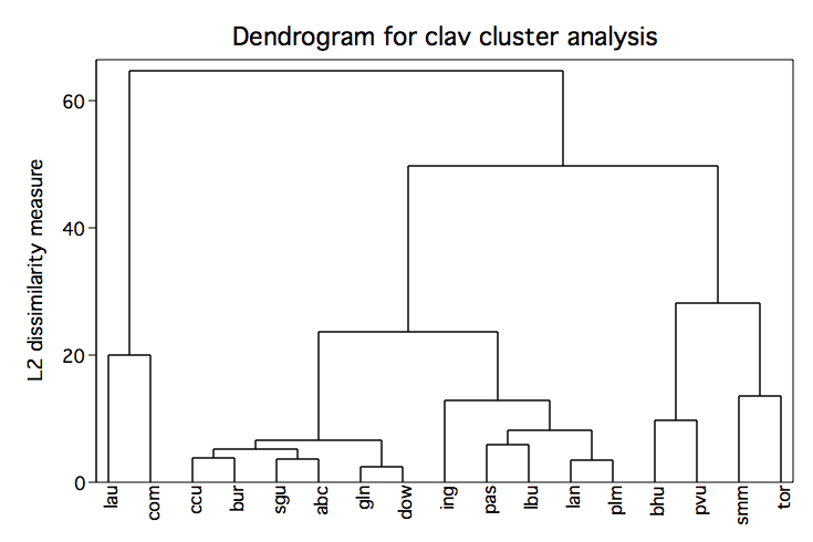
input lep read math lang str3 district
.38 626.5 601.3 605.3 lau
.18 654.0 647.1 641.8 ccu
.07 677.2 676.5 670.5 bhu
.09 639.9 640.3 636.0 ing
.19 614.7 617.3 606.2 com
.12 670.2 666.0 659.3 smm
.20 651.1 645.2 643.4 bur
.41 645.4 645.8 644.8 gln
.07 683.5 682.9 674.3 pvu
.39 648.6 647.8 643.1 sgu
.21 650.4 650.8 643.9 abc
.24 637.0 636.9 626.5 pas
.09 641.1 628.8 629.4 lan
.12 638.0 627.7 628.6 plm
.11 661.4 659.0 651.8 tor
.22 646.4 646.2 647.0 dow
.33 634.1 632.0 627.8 lbu
end

cluster average lep read math lang, name(clav)

cluster tree clav, label(district) xlabel(,angle(90))
cluster gen ave4=groups(4)

sort ave4

list ave4 district, sepby(ave4) noobs

  +-----------------+
  | ave4   district |
  |-----------------|
  |    1        lau |
  |    1        com |
  |-----------------|
  |    2        bhu |
  |    2        pvu |
  |-----------------|
  |    3        tor |
  |    3        smm |
  |-----------------|
  |    4        ccu |
  |    4        plm |
  |    4        sgu |
  |    4        abc |
  |    4        lan |
  |    4        gln |
  |    4        bur |
  |    4        dow |
  |    4        lbu |
  |    4        pas |
  |    4        ing |
  +-----------------+
Complete Linkage Cluster Analysis in Stata
cluster complete lep read math lang, name(clcom)

cluster tree clcom, label(district) xlabel(,angle(90))
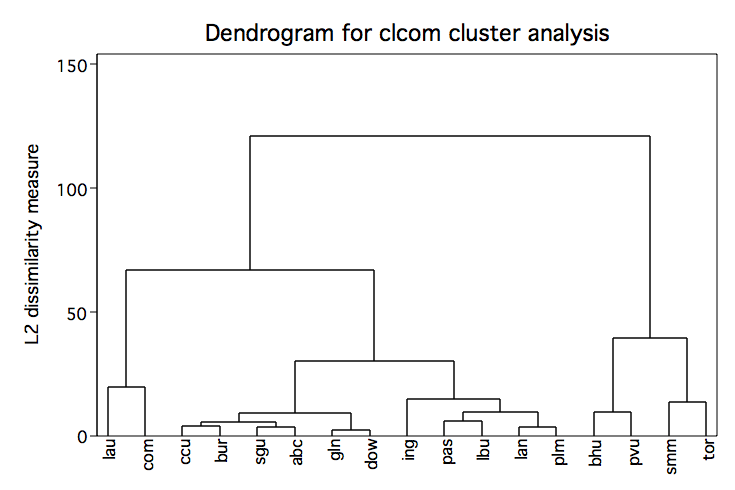
cluster gen com4=groups(4)

sort com4

list com4 district, sepby(com4) noobs

  +-----------------+
  | com4   district |
  |-----------------|
  |    1        com |
  |    1        lau |
  |-----------------|
  |    2        abc |
  |    2        sgu |
  |    2        lan |
  |    2        plm |
  |    2        dow |
  |    2        pas |
  |    2        ccu |
  |    2        ing |
  |    2        bur |
  |    2        gln |
  |    2        lbu |
  |-----------------|
  |    3        bhu |
  |    3        pvu |
  |-----------------|
  |    4        tor |
  |    4        smm |
  +-----------------+
Single Linkage Cluster Analysis in Stata
cluster single lep read math lang, name(clsin)

cluster tree clsin, label(district) xlabel(,angle(90))
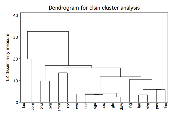
cluster gen sin4=groups(4)

sort sin4

list sin4 district, sepby(sin4) noobs

  +-----------------+
  | sin4   district |
  |-----------------|
  |    1        com |
  |-----------------|
  |    2        lau |
  |-----------------|
  |    3        pvu |
  |    3        bhu |
  |-----------------|
  |    4        gln |
  |    4        dow |
  |    4        pas |
  |    4        lan |
  |    4        abc |
  |    4        tor |
  |    4        ccu |
  |    4        bur |
  |    4        sgu |
  |    4        ing |
  |    4        lbu |
  |    4        smm |
  |    4        plm |
  +-----------------+
Ward's Method Cluster Analysis in Stata
cluster wards lep read math lang, name(clwar)

cluster tree clwar, label(district) xlabel(,angle(90))
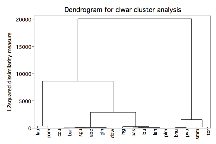
cluster gen ward4=groups(4)

sort ward4

list ward4 district, sepby(ward4) noobs

  +------------------+
  | ward4   district |
  |------------------|
  |     1        com |
  |     1        lau |
  |------------------|
  |     2        gln |
  |     2        dow |
  |     2        abc |
  |     2        bur |
  |     2        sgu |
  |     2        ccu |
  |------------------|
  |     3        lan |
  |     3        lbu |
  |     3        pas |
  |     3        ing |
  |     3        plm |
  |------------------|
  |     4        pvu |
  |     4        bhu |
  |     4        smm |
  |     4        tor |
  +------------------+

tabstat lep read math lang, by(ward4) stat(n mean sd)

Summary statistics: N, mean, sd
  by categories of: ward4

   ward4 |       lep      read      math      lang
---------+----------------------------------------
       1 |         2         2         2         2
         |      .285     620.6     609.3    605.75
         |  .1343503  8.343851  11.31371  .6364134
---------+----------------------------------------
       2 |         6         6         6         6
         |  .2683333  649.3167    647.15       644
         |  .1030372  3.182703  2.013696  1.769748
---------+----------------------------------------
       3 |         5         5         5         5
         |      .174    638.02    633.14    629.66
         |  .1069112  2.712385  5.364979  3.702434
---------+----------------------------------------
       4 |         4         4         4         4
         |     .0925   673.075     671.1   663.975
         |  .0262996  9.491522  10.65865  10.31613
---------+----------------------------------------
   Total |        17        17        17        17
         |  .2011765  648.2059  644.2118  639.9824
         |  .1148304  17.57874  20.30782  18.81831
--------------------------------------------------

xi: mvreg lep read math lang = i.ward4
i.ward4           _Iward4_1-4         (naturally coded; _Iward4_1 omitted)

Equation          Obs  Parms        RMSE    "R-sq"          F        P
----------------------------------------------------------------------
lep                17      4    .0956469    0.4363   3.353913   0.0523
read               17      4    5.683735    0.9151   46.68266   0.0000
math               17      4    6.817553    0.9084   42.98923   0.0000
lang               17      4    5.478383    0.9311   58.59633   0.0000

------------------------------------------------------------------------------
             |      Coef.   Std. Err.      t    P>|t|     [95% Conf. Interval]
-------------+----------------------------------------------------------------
lep          |
   _Iward4_2 |  -.0166667   .0780954    -0.21   0.834    -.1853815    .1520482
   _Iward4_3 |      -.111    .080024    -1.39   0.189    -.2838812    .0618812
   _Iward4_4 |     -.1925   .0828327    -2.32   0.037    -.3714491   -.0135509
       _cons |       .285   .0676326     4.21   0.001     .1388887    .4311113
-------------+----------------------------------------------------------------
read         |
   _Iward4_2 |   28.71666    4.64075     6.19   0.000     18.69093     38.7424
   _Iward4_3 |   17.41999   4.755354     3.66   0.003     7.146672    27.69331
   _Iward4_4 |   52.47501   4.922259    10.66   0.000     41.84111     63.1089
       _cons |      620.6   4.019007   154.42   0.000     611.9175    629.2825
-------------+----------------------------------------------------------------
math         |
   _Iward4_2 |   37.85001   5.566509     6.80   0.000     25.82429    49.87572
   _Iward4_3 |   23.84001   5.703974     4.18   0.001     11.51733     36.1627
   _Iward4_4 |   61.80002   5.904174    10.47   0.000     49.04483    74.55521
       _cons |      609.3   4.820738   126.39   0.000     598.8854    619.7146
-------------+----------------------------------------------------------------
lang         |
   _Iward4_2 |      38.25   4.473081     8.55   0.000      28.5865     47.9135
   _Iward4_3 |      23.91   4.583544     5.22   0.000     14.00785    33.81214
   _Iward4_4 |   58.22499   4.744419    12.27   0.000      47.9753    68.47468
       _cons |     605.75   3.873802   156.37   0.000     597.3812    614.1188
------------------------------------------------------------------------------
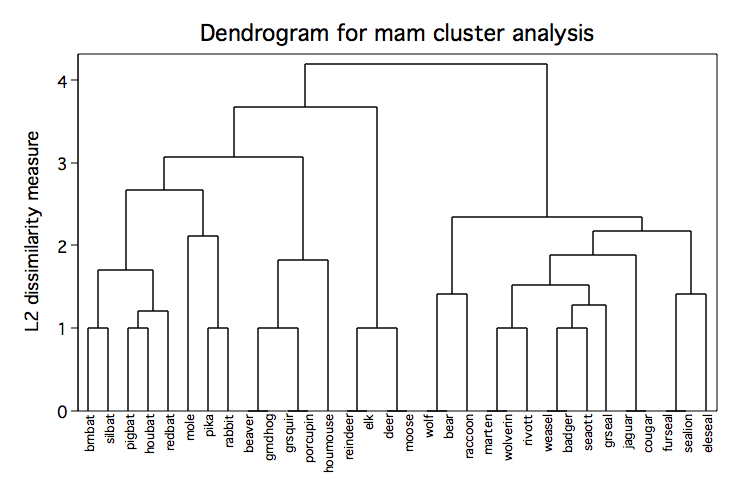
Average Linkage Cluster Analysis for Mammal Data
use http://www.gseis.ucla.edu/courses/data/mammal, clear

format v1- v8 %2.0f

list ,noobs nodis

   mammal  v1  v2  v3  v4  v5  v6  v7  v8
   brnbat   2   3   1   1   3   3   3   3
     mole   3   2   1   0   3   3   3   3
   silbat   2   3   1   1   2   3   3   3
   pigbat   2   3   1   1   2   2   3   3
   houbat   2   3   1   1   1   2   3   3
   redbat   1   3   1   1   1   2   3   3
     pika   2   1   0   0   2   2   3   3
   rabbit   2   1   0   0   3   2   3   3
   beaver   1   1   0   0   2   1   3   3
  grndhog   1   1   0   0   2   1   3   3
  grsquir   1   1   0   0   1   1   3   3
 houmouse   1   1   0   0   0   0   3   3
 porcupin   1   1   0   0   1   1   3   3
     wolf   3   3   1   1   4   4   2   3
     bear   3   3   1   1   4   4   2   3
  raccoon   3   3   1   1   4   4   3   2
   marten   3   3   1   1   4   4   1   2
   weasel   3   3   1   1   3   3   1   2
 wolverin   3   3   1   1   4   4   1   2
   badger   3   3   1   1   3   3   1   2
   rivott   3   3   1   1   4   3   1   2
   seaott   3   2   1   1   3   3   1   2
   jaguar   3   3   1   1   3   2   1   1
   cougar   3   3   1   1   3   2   1   1
  furseal   3   2   1   1   4   4   1   1
  sealion   3   2   1   1   4   4   1   1
   grseal   3   2   1   1   3   3   2   2
  eleseal   2   1   1   1   4   4   1   1
 reindeer   0   4   1   0   3   3   3   3
      elk   0   4   1   0   3   3   3   3
     deer   0   4   0   0   3   3   3   3
    moose   0   4   0   0   3   3   3   3

cluster average v1- v8, name(mam)

cluster tree mam, label(mammal) xlabel(,angle(90) labsize(*.75))
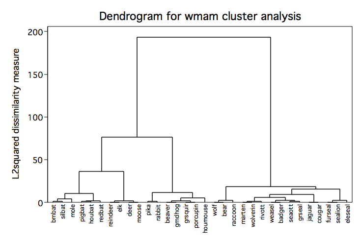
Ward's Method Cluster Analysis for Mammal Data
cluster wards v1- v8, name(wmam)

cluster tree wmam, label(mammal) xlabel(,angle(90) labsize(*.75))
Example Using Fisher Iris Data
use http://www.gseis.ucla.edu/courses/data/iris

cluster average sl sw pl pw, name(c1)

cluster gen c1=groups(3), name(c1)

tabulate c1 type

           |           type of iris
        c1 |    setosa  versicolo  virginica |     Total
-----------+---------------------------------+----------
         1 |        50          0          0 |        50
         2 |         0         50         14 |        64
         3 |         0          0         36 |        36
-----------+---------------------------------+----------
     Total |        50         50         50 |       150

cluster wards sl sw pl pw, name(wcl)

cluster gen wcl=groups(3), name(wcl)

tabulate wcl type

           |           type of iris
       wcl |    setosa  versicolo  virginica |     Total
-----------+---------------------------------+----------
         1 |        50          0          0 |        50
         2 |         0         49         15 |        64
         3 |         0          1         35 |        36
-----------+---------------------------------+----------
     Total |        50         50         50 |       150

tabulate c1 wcl

           |                wcl
        c1 |         1          2          3 |     Total
-----------+---------------------------------+----------
         1 |        50          0          0 |        50
         2 |         0         63          1 |        64
         3 |         0          1         35 |        36
-----------+---------------------------------+----------
     Total |        50         64         36 |       150
The Ward's method and average linkage clustering produce almost identical clusters for
the Fisher Iris data.
Multivariate Course Page
Phil Ender, 29Jan98