*May Require Technology Fee
**Social Science students only
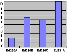
Relative Course Difficulty

Let's get started...
What makes a model multivariate?
Instructor: Phil Ender
Textbook:
You can view textbook examples for this book using several different statistical software packages at the ATS website: Afifi, Clark & May -- Textbook Examples.
Topics Covered by Afifi et al vs Lecture
Textbook                          Lecture
                                  matrix algebra
simple linear regression          simple linear regression
multiple linear regression        multiple linear regression
                                  multivariate multiple regression
                                  Hotellings T2
                                  multivariate analysis of variance
canonical correlation             canonical correlation
discriminant analysis             discriminant analysis
logistic regression               probit regression
survival analysis
principal components analysis     principal components analysis
factor analysis                   factor analysis
cluster analysis                  cluster analysis
log-linear analysis
Course Organization
Electronic Support
Multivariate Course Webpage
Lecture Notes
About Assignments
Computers Running Stata
*May Require Technology Fee
**Social Science students only
Relative Course Difficulty

Let's get started...
What makes a model multivariate?
Every model has a
Here are two univariate models.
The concept of right hand side and left hand side equivalence.
There are times when rhs variables and lhs variables an be exchanged and the two models can yield the same results.
/* multivariate anova -- female is a rhs variable */
manova read write math = female

                           Number of obs =     200

                           W = Wilks' lambda      L = Lawley-Hotelling trace
                           P = Pillai's trace     R = Roy's largest root

                  Source |  Statistic     df   F(df1,    df2) =   F   Prob>F
              -----------+--------------------------------------------------
                  female | W   0.8501      1     3.0   196.0    11.52 0.0000 e
                         | P   0.1499            3.0   196.0    11.52 0.0000 e
                         | L   0.1763            3.0   196.0    11.52 0.0000 e
                         | R   0.1763            3.0   196.0    11.52 0.0000 e
                         |--------------------------------------------------
                Residual |               198
              -----------+--------------------------------------------------
                   Total |               199
              --------------------------------------------------------------
                           e = exact, a = approximate, u = upper bound on F

/* OLS regression -- female is a lhs variable */
/* in SAS: model female = read write math     */
regress female read write math

      Source |       SS       df       MS              Number of obs =     200
-------------+------------------------------           F(  3,   196) =   11.52
       Model |  7.43351627     3  2.47783876           Prob > F      =  0.0000
    Residual |  42.1614837   196  .215109611           R-squared     =  0.1499
-------------+------------------------------           Adj R-squared =  0.1369
       Total |      49.595   199  .249221106           Root MSE      =   .4638

------------------------------------------------------------------------------
      female |      Coef.   Std. Err.      t    P>|t|     [95% Conf. Interval]
-------------+----------------------------------------------------------------
        read |  -.0112975   .0045153    -2.50   0.013    -.0202023   -.0023926
       write |   .0270844   .0046522     5.82   0.000     .0179095    .0362593
        math |  -.0102947   .0050408    -2.04   0.042     -.020236   -.0003535
       _cons |   .2476519   .2099033     1.18   0.239    -.1663071     .661611
------------------------------------------------------------------------------
The role of matrix algebra in multivariate analysis.Matrix algebra gives us a concise and elegant way in which to represent multivariate models. If you are intimidated by it, please realize that the alternatives to matrix representation are worse.
Consider this univariate multiple regression model
These examples are in stat package pseudo-code
Regression:
model       y  = x1            /* simple linear regression */
model       y  = x1 x2 x3      /* multiple linear regression */
model y1 y2 y3 = x1 x2 x3      /* multivariate multiple regression */

Probit Analysis (the z's are binary, 0/1, variables):
model       z  = x1            /* simple probit analysis */
model       z  = x1 x2 x3      /* multiple probit analysis */
model z1 z2 z3 = x1 x2 x3      /* multivariate probit analysis */

Correlation:
model           ry,x           /* Pearson correlation */
model           Ry.x1,x2,x3    /* multiple correlation */
model RC y1,y2,y3 = x1,x2,x3   /* cannonical correlation */

Anova:
model       y  = a             /* one-way anova */
model       y  = a b a*b       /* two-way anova */
model y1 y2 y3 = a             /* one-way multivariate anova (manova) */
model y1 y2 y3 = a b a*b       /* two-way multivariate anova (manova) */
Classifying Multivariate Models
I. Testing effects; discriminating among groups
anova -> manova
multiple linear regression -> multivariate multiple regression
multiple linear regression -> canonical correlation analysis
Examples:
ttest write, by(female)

Two-sample t test with equal variances

------------------------------------------------------------------------------
   Group |     Obs        Mean    Std. Err.   Std. Dev.   [95% Conf. Interval]
---------+--------------------------------------------------------------------
    male |      91    50.12088    1.080274    10.30516    47.97473    52.26703
  female |     109    54.99083    .7790686    8.133715    53.44658    56.53507
---------+--------------------------------------------------------------------
combined |     200      52.775    .6702372    9.478586    51.45332    54.09668
---------+--------------------------------------------------------------------
    diff |           -4.869947    1.304191               -7.441835   -2.298059
------------------------------------------------------------------------------
Degrees of freedom: 198

                  Ho: mean(male) - mean(female) = diff = 0

     Ha: diff < 0               Ha: diff != 0              Ha: diff > 0
       t =  -3.7341                t =  -3.7341              t =  -3.7341
   P < t =   0.0001          P > |t| =   0.0002          P > t =   0.9999

hotel write, by(female) notable

2-group Hotelling's T-squared = 13.943308
F test statistic: ((200-1-1)/(200-2)(1)) x 13.943308 = 13.943308

H0: Vectors of means are equal for the two groups
              F(1,198) =   13.9433
       Prob > F(1,198) =    0.0002

display sqrt(r(T2))
3.7340739

anova write prog

                           Number of obs =     200     R-squared     =  0.1776
                           Root MSE      = 8.63918     Adj R-squared =  0.1693

                  Source |  Partial SS    df       MS           F     Prob > F
              -----------+----------------------------------------------------
                   Model |  3175.69786     2  1587.84893      21.27     0.0000
                         |
                    prog |  3175.69786     2  1587.84893      21.27     0.0000
                         |
                Residual |  14703.1771   197   74.635417
              -----------+----------------------------------------------------
                   Total |   17878.875   199   89.843593

manova write = prog

                           Number of obs =     200

                           W = Wilks' lambda      L = Lawley-Hotelling trace
                           P = Pillai's trace     R = Roy's largest root

                  Source |  Statistic     df   F(df1,    df2) =   F   Prob>F
              -----------+--------------------------------------------------
                    prog | W   0.8224      2     2.0   197.0    21.27 0.0000 e
                         | P   0.1776            2.0   197.0    21.27 0.0000 e
                         | L   0.2160            2.0   197.0    21.27 0.0000 e
                         | R   0.2160            2.0   197.0    21.27 0.0000 e
                         |--------------------------------------------------
                Residual |               197
              -----------+--------------------------------------------------
                   Total |               199
              --------------------------------------------------------------
                           e = exact, a = approximate, u = upper bound on F

regress write read female

      Source |       SS       df       MS              Number of obs =     200
-------------+------------------------------           F(  2,   197) =   77.21
       Model |  7856.32118     2  3928.16059           Prob > F      =  0.0000
    Residual |  10022.5538   197  50.8759077           R-squared     =  0.4394
-------------+------------------------------           Adj R-squared =  0.4337
       Total |   17878.875   199   89.843593           Root MSE      =  7.1327

------------------------------------------------------------------------------
       write |      Coef.   Std. Err.      t    P>|t|     [95% Conf. Interval]
-------------+----------------------------------------------------------------
        read |   .5658869   .0493849    11.46   0.000      .468496    .6632778
      female |   5.486894   1.014261     5.41   0.000      3.48669    7.487098
       _cons |   20.22837   2.713756     7.45   0.000     14.87663    25.58011
------------------------------------------------------------------------------

display sqrt(.4394192130387506) /* multiple correlation */

.66288703

mvreg write = read female

Equation          Obs  Parms        RMSE    "R-sq"          F        P
----------------------------------------------------------------------
write             200      3    7.132735    0.4394   77.21062   0.0000

------------------------------------------------------------------------------
             |      Coef.   Std. Err.      t    P>|t|     [95% Conf. Interval]
-------------+----------------------------------------------------------------
write        |
        read |   .5658869   .0493849    11.46   0.000      .468496    .6632778
      female |   5.486894   1.014261     5.41   0.000      3.48669    7.487098
       _cons |   20.22837   2.713756     7.45   0.000     14.87663    25.58011
------------------------------------------------------------------------------


canon (write) (read female)

Linear combinations for canonical correlation 1        Number of obs =     200
------------------------------------------------------------------------------
             |      Coef.   Std. Err.      t    P>|t|     [95% Conf. Interval]
-------------+----------------------------------------------------------------
u            |
       write |    .105501   .0084684    12.46   0.000     .0888016    .1222004
-------------+----------------------------------------------------------------
v            |
        read |    .090063   .0078598    11.46   0.000     .0745639    .1055622
      female |   .8732598   .1614235     5.41   0.000     .5549397     1.19158
------------------------------------------------------------------------------
                                     (Standard errors estimated conditionally)
Canonical correlations:
  0.6629

display .66288703^2  /* canonical correlation squared */

.43941921
Multivariate Course Page
Phil Ender, 12jul07, 30sep05, 24jan05