Linear Statistical Models: Regression
Product Variables and Interactions
Updated for Stata 11
Product Variables
Product variables are created by multiplying one variable times another
and using the product as a predictor variable in a regression analysis.
Example: fXr = female * read
Interactions
Some researchers think that all product variables are interactions. Others restrict the
use of the term interaction to those product variables that are formed in fixed-effects
(anova type) models.
Whether you believe that all product variables are interactions or not, it is the case that
all interations can be concieved of as product variables.
Stata Example
We will use the htwt dataset to illustrate the product variables.
use http://www.philender.com/courses/data/htwt, clear

describe

Contains data from http://www.gseis.ucla.edu/courses/data/htwt.dta
  obs:         1,000                          NCDS Data
 vars:             4                          12 Feb 2001 08:32
 size:        20,000 (99.6% of memory free)
-------------------------------------------------------------------------------
   1. female    float  %9.0g       sl         Sex
   2. height    float  %9.0g                  Height at Age 16 in Centimeters
   3. weight    float  %9.0g                  Weight at Age 16 in Kilograms
   4. mal       float  %9.0g                  Malaise Score at Age 22
-------------------------------------------------------------------------------

summarize

Variable |     Obs        Mean   Std. Dev.       Min        Max
---------+-----------------------------------------------------
  female |    1000        .509   .5001691          0          1
  height |    1000     166.163   8.025138        144        189
  weight |    1000    57.17209   9.656277      34.92     111.36
     mal |    1000       2.591   2.842851          0         19

regress weight female height

  Source |       SS       df       MS                  Number of obs =    1000
---------+------------------------------               F(  2,   997) =  187.77
   Model |    25486.61     2   12743.305               Prob > F      =  0.0000
Residual |  67663.8236   997  67.8674259               R-squared     =  0.2736
---------+------------------------------               Adj R-squared =  0.2721
   Total |  93150.4336   999  93.2436773               Root MSE      =  8.2382

------------------------------------------------------------------------------
  weight |      Coef.   Std. Err.       t     P>|t|       [95% Conf. Interval]
---------+--------------------------------------------------------------------
  female |   1.343864   .6250126      2.150   0.032       .1173726    2.570355
  height |   .6717493   .0389541     17.245   0.000       .5953079    .7481908
   _cons |  -55.13182   6.658765     -8.280   0.000      -68.19863   -42.06502
------------------------------------------------------------------------------

predict p1

sort female height

graph twoway scatter weight p1 height, msym(oh i) con(. L) jitter(1) legend(off)


regress weight i.female##c.height

      Source |       SS       df       MS              Number of obs =    1000
-------------+------------------------------           F(  3,   996) =  128.78
       Model |  26034.4351     3  8678.14505           Prob > F      =  0.0000
    Residual |  67115.9985   996  67.3855406           R-squared     =  0.2795
-------------+------------------------------           Adj R-squared =  0.2773
       Total |  93150.4336   999  93.2436773           Root MSE      =  8.2089

------------------------------------------------------------------------------
      weight |      Coef.   Std. Err.      t    P>|t|     [95% Conf. Interval]
-------------+----------------------------------------------------------------
    1.female |   38.26321   12.96338     2.95   0.003     12.82455    63.70188
      height |   .7706638    .052059    14.80   0.000     .6685058    .8728217
             |
      female#|
    c.height |
          1  |  -.2227448   .0781214    -2.85   0.004    -.3760463   -.0694434
             |
       _cons |  -72.01376   8.892743    -8.10   0.000    -89.46442   -54.56309
------------------------------------------------------------------------------

twoway (scatter weight height, msym(Oh) jitter(2))(lfit weight height if ~female) ///
(lfit weight height if female), legend(off)
regress weight i.female##c.height
Source | SS df MS Number of obs = 1000
-------------+------------------------------ F( 3, 996) = 128.78
Model | 26034.4351 3 8678.14505 Prob > F = 0.0000
Residual | 67115.9985 996 67.3855406 R-squared = 0.2795
-------------+------------------------------ Adj R-squared = 0.2773
Total | 93150.4336 999 93.2436773 Root MSE = 8.2089
------------------------------------------------------------------------------
weight | Coef. Std. Err. t P>|t| [95% Conf. Interval]
-------------+----------------------------------------------------------------
1.female | 38.26321 12.96338 2.95 0.003 12.82455 63.70188
height | .7706638 .052059 14.80 0.000 .6685058 .8728217
|
female#|
c.height |
1 | -.2227448 .0781214 -2.85 0.004 -.3760463 -.0694434
|
_cons | -72.01376 8.892743 -8.10 0.000 -89.46442 -54.56309
------------------------------------------------------------------------------
twoway (scatter weight height, msym(Oh) jitter(2))(lfit weight height if ~female) ///
(lfit weight height if female), legend(off)
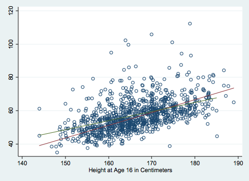
Interpreting the Product Variable
One way of interpreting the product variable is to think of it as examining the the difference
in the regression slopes for, in this instance, males and females. Here is what
the separate regressions would look like in Stata.
sort female

by female: regress weight height

-> female = male

      Source |       SS       df       MS              Number of obs =     491
-------------+------------------------------           F(  1,   489) =  205.86
       Model |  14767.4161     1  14767.4161           Prob > F      =  0.0000
    Residual |  35077.9966   489  71.7341443           R-squared     =  0.2963
-------------+------------------------------           Adj R-squared =  0.2948
       Total |  49845.4127   490  101.725332           Root MSE      =  8.4696

------------------------------------------------------------------------------
      weight |      Coef.   Std. Err.      t    P>|t|     [95% Conf. Interval]
-------------+----------------------------------------------------------------
      height |   .7706638   .0537125    14.35   0.000     .6651279    .8761996
       _cons |  -72.01376   9.175196    -7.85   0.000    -90.04143   -53.98608
------------------------------------------------------------------------------

-> female = female

      Source |       SS       df       MS              Number of obs =     509
-------------+------------------------------           F(  1,   507) =   94.36
       Model |  5962.65403     1  5962.65403           Prob > F      =  0.0000
    Residual |  32038.0019   507  63.1913253           R-squared     =  0.1569
-------------+------------------------------           Adj R-squared =  0.1552
       Total |  38000.6559   508  74.8044408           Root MSE      =  7.9493

------------------------------------------------------------------------------
      weight |      Coef.   Std. Err.      t    P>|t|     [95% Conf. Interval]
-------------+----------------------------------------------------------------
      height |   .5479189    .056406     9.71   0.000     .4371007    .6587372
       _cons |  -33.75054   9.134041    -3.70   0.000    -51.69577   -15.80531
------------------------------------------------------------------------------
Note that the regression coefficient for height is significant in each of the two models and that
there is a fairly large difference in the two constants.
Doing the Arithmetic Manually
Let's start with the regression equation from the model with the product variable:
weight' = -72.01 + 38.26*female + .77*height - .22*fxh
When the female = male (female = 0), the formula above reduces to:
weight' = -72.01 + 38.26*female + .77*height - .22*female*height
weight' = -72.01 + 38.26*0      + .77*height - .22*0*height
weight' = -72.01 + 38.26*0      + .77*height - 0
weight' = -72.01                + .77*height
Now when female = female (female=1), the formula above reduces to:
weight' = -72.01 + 38.26*female + .77*height - .22*female*height
weight' = -72.01 + 38.26*1      + .77*height - .22*1*height
weight' = -72.01 + 38.26        + .77*height - .22*height
weight' = -33.75                + .55*height
In this example, short females tend to be heavier that corresponding males but tall females
tend to be lighter.
Example 2
This time we will create the interaction on the fly.
use http://www.philender.com/courses/data/hsbdemo, clear

regress write i.female##c.socst


      Source |       SS       df       MS              Number of obs =     200
-------------+------------------------------           F(  3,   196) =   49.26
       Model |  7685.43528     3  2561.81176           Prob > F      =  0.0000
    Residual |  10193.4397   196  52.0073455           R-squared     =  0.4299
-------------+------------------------------           Adj R-squared =  0.4211
       Total |   17878.875   199   89.843593           Root MSE      =  7.2116

------------------------------------------------------------------------------
       write |      Coef.   Std. Err.      t    P>|t|     [95% Conf. Interval]
-------------+----------------------------------------------------------------
    1.female |   15.00001    5.09795     2.94   0.004     4.946132    25.05389
       socst |   .6247968   .0670709     9.32   0.000     .4925236    .7570701
             |
      female#|
     c.socst |
          1  |  -.2047288   .0953726    -2.15   0.033    -.3928171   -.0166405
             |
       _cons |    17.7619   3.554993     5.00   0.000     10.75095    24.77284
------------------------------------------------------------------------------
Here is the interpretation of each of the terms in the model.
_cons = 17.7619 -- This is the expected value when female = 0 (males) and
socst = 0.
1.female = 15.00001 -- This is how much the expected value will increase when
female = 1 (females) and socst = 0 (15.00001 + 17.7619 = 32.76191).
socst = .6247968 -- This is the slope for write regressed on read
when female = 0 (males).
female#c.socst = -.2047288 -- This is how the the slope will change when
female = 1 (females) (.6247968 - .2047288 = .420068).
This can be shown by running separate regressions for males and females.
bysort female: regress write socst

-> female=     male
  Source |       SS       df       MS                  Number of obs =      91
---------+------------------------------               F(  1,    89) =   79.62
   Model |  4513.09285     1  4513.09285               Prob > F      =  0.0000
Residual |  5044.57748    89  56.6806458               R-squared     =  0.4722
---------+------------------------------               Adj R-squared =  0.4663
   Total |  9557.67033    90  106.196337               Root MSE      =  7.5287

------------------------------------------------------------------------------
   write |      Coef.   Std. Err.       t     P>|t|       [95% Conf. Interval]
---------+--------------------------------------------------------------------
   socst |   .6247968   .0700195      8.923   0.000       .4856696    .7639241
   _cons |    17.7619   3.711281      4.786   0.000       10.38766    25.13613
------------------------------------------------------------------------------

-> female=   female
  Source |       SS       df       MS                  Number of obs =     109
---------+------------------------------               F(  1,   107) =   41.48
   Model |  1996.12858     1  1996.12858               Prob > F      =  0.0000
Residual |  5148.86224   107  48.1202079               R-squared     =  0.2794
---------+------------------------------               Adj R-squared =  0.2726
   Total |  7144.99083   108  66.1573225               Root MSE      =  6.9369

------------------------------------------------------------------------------
   write |      Coef.   Std. Err.       t     P>|t|       [95% Conf. Interval]
---------+--------------------------------------------------------------------
   socst |    .420068   .0652213      6.441   0.000       .2907745    .5493615
   _cons |    32.7619   3.514715      9.321   0.000       25.79439    39.72942
------------------------------------------------------------------------------
Doing the Arithmetic Manually
Let's start with the regression equation from the model with the product variable:
write' = 17.76 + .625*socst + 15.*female - .205*fXs
When the female = male (female = 0), the formula above reduces to:
write' = 17.76 + .625*socst + 15*0 - .205*0*socst
write' = 17.76 + .625*socst + 0    - 0
write' = 17.76 + .625*socst
Now when female = female (female=1), the formula above reduces to:
write' = 17.76 + .625*socst + 15.*1 - .205*1*socst
write' = 17.76 + .625*socst + 15.   - .205*socst
write' = 32.76 + .42*socst
Solving for the Crossing Point
Set the male equation equal to the female equation and solve for socst.
17.76 + .625*socst + 15*0 - .205*0*socst = 17.76 + .625*socst + 15*1 - .205*1*socst
17.76 + .625*socst = 17.76 + .625*socst + 15 - .205*socst
17.76 - 17.76 + .625*socst - .625*socst = 15 - .205*socst
0 = 15 - .205*socst
.205*socst = 15
socst = 15/.205
socst = 73.170732
Thus, when socst = 73.170732 the predicted write scores for males and females are equal.
When socst < 73.170732 the predicted write score for females is greater than for
males and when socst > 73.170732 the predicted score for males is greater than for
females.
Another Example
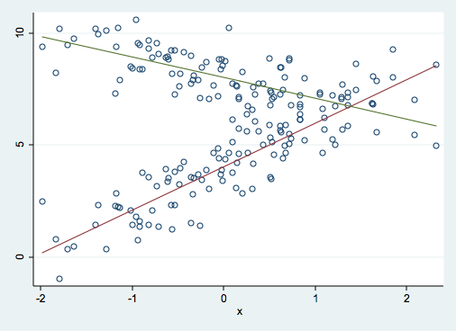
use http://www.philender.com/courses/data/reginteraction, clear

describe

Contains data from reginteraction.dta
  obs:           200
 vars:             4                          27 Oct 2004 11:31
 size:         4,000 (99.9% of memory free)
-------------------------------------------------------------------------------
              storage  display     value
variable name   type   format      label      variable label
-------------------------------------------------------------------------------
id              float  %9.0g
y               float  %9.0g
x               float  %9.0g
grp             float  %9.0g                  0/1 variable
-------------------------------------------------------------------------------

tab grp

        0/1 |
   variable |      Freq.     Percent        Cum.
------------+-----------------------------------
          0 |        100       50.00       50.00
          1 |        100       50.00      100.00
------------+-----------------------------------
      Total |        200      100.00

univar y x
                                        -------------- Quantiles --------------
Variable       n     Mean     S.D.      Min      .25      Mdn      .75      Max
-------------------------------------------------------------------------------
       y     200     6.04     2.57    -0.95     3.97     6.72     8.04    10.59
       x     200     0.03     0.93    -1.98    -0.63     0.04     0.66     2.32
-------------------------------------------------------------------------------

/* regression for whole sample */

regress y x

      Source |       SS       df       MS              Number of obs =     200
-------------+------------------------------           F(  1,   198) =    6.91
       Model |  44.2818817     1  44.2818817           Prob > F      =  0.0092
    Residual |  1268.60934   198   6.4071179           R-squared     =  0.0337
-------------+------------------------------           Adj R-squared =  0.0288
       Total |  1312.89123   199  6.59744335           Root MSE      =  2.5312

------------------------------------------------------------------------------
           y |      Coef.   Std. Err.      t    P>|t|     [95% Conf. Interval]
-------------+----------------------------------------------------------------
           x |   .5068139   .1927822     2.63   0.009     .1266441    .8869837
       _cons |   6.025549   .1790882    33.65   0.000     5.672384    6.378714
------------------------------------------------------------------------------

/* regression with categorical variable but no interaction */

regress y x grp

      Source |       SS       df       MS              Number of obs =     200
-------------+------------------------------           F(  2,   197) =  155.18
       Model |  803.114016     2  401.557008           Prob > F      =  0.0000
    Residual |  509.777211   197  2.58770158           R-squared     =  0.6117
-------------+------------------------------           Adj R-squared =  0.6078
       Total |  1312.89123   199  6.59744335           Root MSE      =  1.6086

------------------------------------------------------------------------------
           y |      Coef.   Std. Err.      t    P>|t|     [95% Conf. Interval]
-------------+----------------------------------------------------------------
           x |   .5068139   .1225159     4.14   0.000     .2652028     .748425
         grp |   3.895721   .2274951    17.12   0.000     3.447083    4.344359
       _cons |   4.077688   .1609098    25.34   0.000     3.760361    4.395015
------------------------------------------------------------------------------

/* regression with interaction */

regress y c.x##i.grp

      Source |       SS       df       MS              Number of obs =     200
-------------+------------------------------           F(  3,   196) =  477.60
       Model |  1154.90449     3  384.968163           Prob > F      =  0.0000
    Residual |  157.986737   196  .806054781           R-squared     =  0.8797
-------------+------------------------------           Adj R-squared =  0.8778
       Total |  1312.89123   199  6.59744335           Root MSE      =  .89781

------------------------------------------------------------------------------
           y |      Coef.   Std. Err.      t    P>|t|     [95% Conf. Interval]
-------------+----------------------------------------------------------------
           x |   1.935305   .0967014    20.01   0.000     1.744596    2.126014
       1.grp |   3.985859   .1270422    31.37   0.000     3.735314    4.236404
             |
     grp#c.x |
          1  |  -2.856982   .1367564   -20.89   0.000    -3.126685   -2.587279
             |
       _cons |   4.032619   .0898324    44.89   0.000     3.855457    4.209781
------------------------------------------------------------------------------

lincom x  /*  slope for grp==0 */

 ( 1)  x = 0
------------------------------------------------------------------------------
           y |      Coef.   Std. Err.      t    P>|t|     [95% Conf. Interval]
-------------+----------------------------------------------------------------
         (1) |   1.935305   .0967014    20.01   0.000     1.744596    2.126014


lincom _cons   /*  constant for grp==0 */

 ( 1)  _cons = 0
------------------------------------------------------------------------------
           y |      Coef.   Std. Err.      t    P>|t|     [95% Conf. Interval]
-------------+----------------------------------------------------------------
         (1) |   4.032619   .0898324    44.89   0.000     3.855457    4.209781


lincom x + 1.grp#c.x  /* slope for grp==1  */


 ( 1)  x + 1.grp#c.x = 0

------------------------------------------------------------------------------
           y |      Coef.   Std. Err.      t    P>|t|     [95% Conf. Interval]
-------------+----------------------------------------------------------------
         (1) |  -.9216771   .0967014    -9.53   0.000    -1.112386   -.7309683

lincom _cons + 1.grp  /*  constant for grp==1  */

 ( 1)  1.grp + _cons = 0

------------------------------------------------------------------------------
           y |      Coef.   Std. Err.      t    P>|t|     [95% Conf. Interval]
-------------+----------------------------------------------------------------
         (1) |   8.018478   .0898324    89.26   0.000     7.841316     8.19564

twoway (scatter y x, msym(Oh))(lfit y x if grp==0)(lfit y x if grp==1), legend(off)
Linear Statistical Models
Phil Ender, 20sep10, 4may06, 3feb04; 14jan00