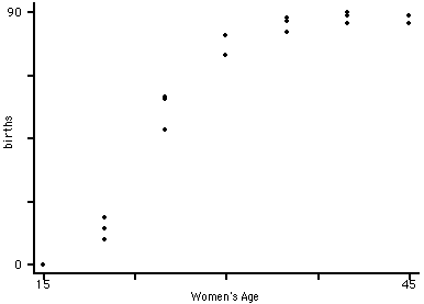
Check out the scatterplot below showing the relationship between a women's age and the percent of women that have children.
It is immediately obvious that the relationship is nonlinear. Furthermore, it is unlikely that any simple power (polynomial) function of age would make the association linear. This is a case for nonlinear regression.
It is possible to fit arbitrary nonlinear functions using least squares. The fitting process is iterative and the process has many things in common with linear regression. The biggest difference is that you need to specify the specific function to be fitted. Usually, there will be some sound theoretical mechanism which specifies the function, however, it is possible to select the function empirically.
Stata has a nonlinear regression command, nl, that works with any user specified function or one of seven built-in functions (3 exponential functions, 2 logistic functions, and 2 Gompertz functions). The dataset on births will be fit using a 3 parameter Gompertz functions:
Here is what the process looks like.
use http://www.philender.com/courses/data/nlex1, clear
list
age births
1. 15 0
2. 20 9
3. 25 48
4. 30 75
5. 35 83
6. 40 86
7. 45 86
8. 15 0
9. 20 13
10. 25 59
11. 30 82
12. 35 87
13. 40 89
14. 45 89
15. 15 0
16. 20 17
17. 25 60
18. 30 82
19. 35 88
20. 40 90
nl gom3 births age
(obs = 20)
Iteration 0: residual SS = 2100.188
Iteration 1: residual SS = 1681.729
Iteration 2: residual SS = 212.8445
Iteration 3: residual SS = 183.136
Iteration 4: residual SS = 183.1101
Source | SS df MS Number of obs = 20
---------+------------------------------ F( 3, 17) = 2777.47
Model | 89749.8899 3 29916.63 Prob > F = 0.0000
Residual | 183.110095 17 10.7711821 R-squared = 0.9980
---------+------------------------------ Adj R-squared = 0.9976
Total | 89933 20 4496.65 Root MSE = 3.281948
Res. dev. = 101.0446
3-parameter Gompertz function, births=b1*exp(-exp(-b2*(age-b3)))
------------------------------------------------------------------------------
births | Coef. Std. Err. t P>|t| [95% Conf. Interval]
---------+--------------------------------------------------------------------
b1 | 88.4125 1.290269 68.523 0.000 85.69026 91.13473
b2 | .2872474 .0203612 14.108 0.000 .2442891 .3302058
b3 | 22.2833 .1979394 112.576 0.000 21.86568 22.70091
------------------------------------------------------------------------------
(SE's, P values, CI's, and correlations are asymptotic approximations)
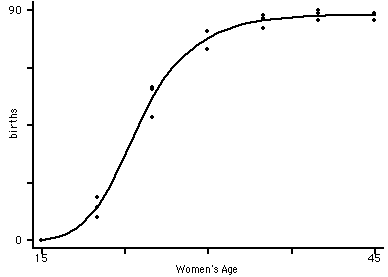
predict p
twoway (scatter births age)(line p age, sort), legend(off) aspect(1)
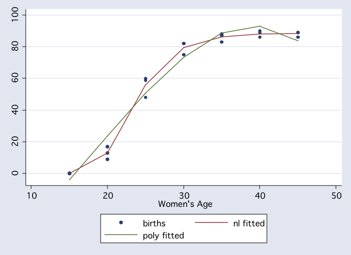
We can compare these results with a polynomial regression of degree three. The R2
is not quite as high and the graph of the predicted values do not fit the observed values
as well as the nonlinear model.
regress births c.age##c.age##c.age

      Source |       SS       df       MS              Number of obs =      20
-------------+------------------------------           F(  3,    16) =  142.02
       Model |  23719.7961     3  7906.59871           Prob > F      =  0.0000
    Residual |  890.753877    16  55.6721173           R-squared     =  0.9638
-------------+------------------------------           Adj R-squared =  0.9570
       Total |    24610.55    19  1295.29211           Root MSE      =  7.4614

------------------------------------------------------------------------------
      births |      Coef.   Std. Err.      t    P>|t|     [95% Conf. Interval]
-------------+----------------------------------------------------------------
         age |   1.161826   6.171481     0.19   0.853    -11.92113    14.24478
             |
 c.age#c.age |   .2399854   .2183397     1.10   0.288    -.2228741    .7028449
             |
 c.age#c.age#|
       c.age |  -.0043201   .0024374    -1.77   0.095    -.0094872    .0008469
             |
       _cons |  -60.90203   54.39825    -1.12   0.279    -176.2212    54.41711
------------------------------------------------------------------------------

predict p2
label variable p2 "poly fitted"
label variable p  "nl fitted"

twoway (scatter births age)(line p age,sort)(line p2 age,sort)