Weighted Least Squares

Linear Statistical Models: Regression

Weighted Least Squares (WLS)

Ordinary least squares (OLS) is the type of regression estimation that we have covered so far in class. OLS, while generally robust, can produce unacceptably high standard errors when the homogeneity of variance assumption is violated. Weighted least squares (WLS) encompases various schemes for weighting observations in order to reduce the effects of heteroscedasticity.

In WLS the goal is to minimize to following sum of squares:

The trick, of course, is determining the values for w_i. According to Miller (1986), "If God or the Devil were willing to tell us the values of w_i...", then the task would be easy.

A Simple Example

From Chatterjee & Price (1977) a study of 27 industrial companies of varying size, recorded the number of workers (x) and the number of supervisors (y). The model y = b_o + b₁x + e was examined.

OLS Analysis

use http://www.philender.com/courses/data/wls, clear

scatter y x, msym(oh)

regress y x

  Source |       SS       df       MS                  Number of obs =      27
---------+------------------------------               F(  1,    25) =   86.54
   Model |  40862.6027     1  40862.6027               Prob > F      =  0.0000
Residual |   11804.064    25   472.16256               R-squared     =  0.7759
---------+------------------------------               Adj R-squared =  0.7669
   Total |  52666.6667    26  2025.64103               Root MSE      =  21.729

------------------------------------------------------------------------------
       y |      Coef.   Std. Err.       t     P>|t|       [95% Conf. Interval]
---------+--------------------------------------------------------------------
       x |   .1053611   .0113256      9.303   0.000       .0820355    .1286867
   _cons |   14.44806   9.562012      1.511   0.143      -5.245273    34.14139
------------------------------------------------------------------------------

rvfplot, yline(0)

Remarks

There is some evidence of heteroscedasity in the x*y plot while the evidence is much stronger in the standardized residual vs x plot.

Since it appears that the variance is increasing as the value of x increases we will try weighting observations by dividing by x.

Here are the transformations:
yt = y/x
xt = 1/x

Now the model becomes yt = b_o + b₁xt + e.

WLS Analysis

generate yt = y/x

generate xt = 1/x

regress yt xt

  Source |       SS       df       MS                  Number of obs =      27
---------+------------------------------               F(  1,    25) =    0.69
   Model |  .000355828     1  .000355828               Prob > F      =  0.4131
Residual |  .012842316    25  .000513693               R-squared     =  0.0270
---------+------------------------------               Adj R-squared = -0.0120
   Total |  .013198144    26  .000507621               Root MSE      =  .02266

------------------------------------------------------------------------------
      yt |      Coef.   Std. Err.       t     P>|t|       [95% Conf. Interval]
---------+--------------------------------------------------------------------
      xt |   3.803296   4.569745      0.832   0.413       -5.60827    13.21486
   _cons |   .1209903   .0089986     13.445   0.000       .1024573    .1395233
------------------------------------------------------------------------------

Remarks

The b_o and b₁ in the WLS are reversed from b_o and b₁ in the OLS.

yt = b_o + b₁xt

(x)yt = (x)b_o + (x)b₁xt [multiply by x]

(x)y/x = (x)b_o + 1/x [substitute for transformed variables]

y = (x)b_o + b₁ [which can be rewritten]

y = b₁x + b₀ = 0.12x + 3.80

Note that the standard errors of the coefficients are smaller for WLS than for OLS.

generate p1 = 3.803296 + .1209903*x

corr p1 y
(obs=27)

             |       p1        y
-------------+------------------
          p1 |   1.0000
           y |   0.8808   1.0000


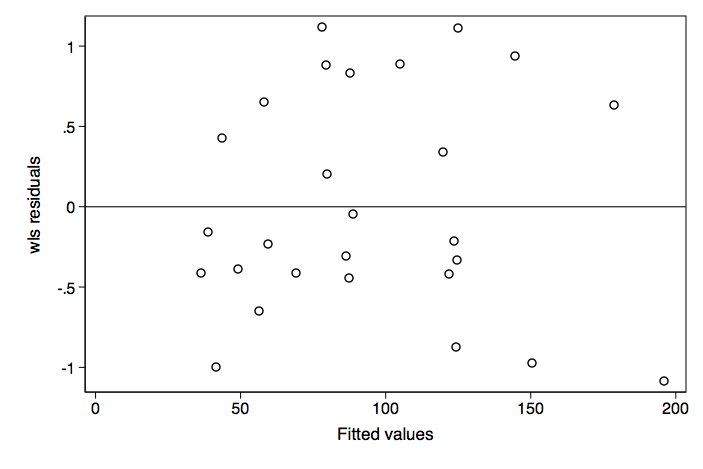
rvfplot, yline(0)

Remarks

Inspection of the residual vs fitted (predicted) plot shows improvement in terms of heteroscedasticity.

WLS the Easy Way

Stata allows us to do WLS through the use of analytic weights, which can be included as part of the regress command.

regress y x [aw = 1/x^2]
(sum of wgt is  1.0470e-004)

  Source |       SS       df       MS                  Number of obs =      27
---------+------------------------------               F(  1,    25) =  180.78
   Model |  23948.6837     1  23948.6837               Prob > F      =  0.0000
Residual |  3311.87511    25  132.475004               R-squared     =  0.8785
---------+------------------------------               Adj R-squared =  0.8737
   Total |  27260.5588    26  1048.48303               Root MSE      =   11.51

------------------------------------------------------------------------------
       y |      Coef.   Std. Err.       t     P>|t|       [95% Conf. Interval]
---------+--------------------------------------------------------------------
       x |   .1209903   .0089986     13.445   0.000       .1024573    .1395233
   _cons |   3.803296   4.569745      0.832   0.413      -5.608271    13.21486
------------------------------------------------------------------------------

The results obtained are the same as going through the process of transforming each of the variables.

More About WLS

There are many other possible weighting schemes:

For example, weighting by sqrt(n)
Using different weights for different subsets of the sample.
And more complex schemes in which the initial OLS is used to derive weights used is a subsequent analysis (two-stage weighted least squares).

Weighted Least Squares using wls0

With wls0 you can use any of the following weighting schemes: 1) abse - absolute value of residual, 2) e2 - residual squared, 3) loge2 - log residual squared, and 4) xb2 - fitted value squared. We will demonstrate the command with the loge2 option.

wls0 y x, wvar(x) type(loge2) graph

WLS regression -  type: proportional to log(e)^2 

(sum of wgt is   1.3388e+00)

      Source |       SS       df       MS              Number of obs =      27
-------------+------------------------------           F(  1,    25) =  128.32
       Model |  36182.5945     1  36182.5945           Prob > F      =  0.0000
    Residual |  7049.36879    25  281.974752           R-squared     =  0.8369
-------------+------------------------------           Adj R-squared =  0.8304
       Total |  43231.9632    26  1662.76782           Root MSE      =  16.792

------------------------------------------------------------------------------
           y |      Coef.   Std. Err.      t    P>|t|     [95% Conf. Interval]
-------------+----------------------------------------------------------------
           x |    .113653   .0100331    11.33   0.000     .0929894    .1343166
       _cons |   8.461635   6.925202     1.22   0.233    -5.801086    22.72436
------------------------------------------------------------------------------

Linear Statistical Models Course

Phil Ender, 20Jun99