Path Analysis

Linear Statistical Models: Regression

Path Analysis

Path Analysis Background

Path analysis represents an early attempt at dealing with causal relationships using regression.
Developed by Sewall Wright in the 1930's.
Currently, causal analysis is done using structural equation modeling.
Path analysis is useful in illustrating a number of the issues involved in causal analysis.

Some Definitions

Exogenous Variable - a variable whose variability is determined by variables outside of the model.
Endogenous Variable - a variable whose variation is explained by either exogenous variables or other (endogenous) variables in the model.
- In a standard multiple regression model the response (dependent) variable is endogenous and the predictors are exogenous.
Recursive Model - a causal model that is unidirectional (one-way causal flow). It has no feedback loops nor any reciprocal effects. In a recursive model, a variable cannot be both cause and effect at the same time.
Nonrecursive Model - a causal model with feedback loops and/or reciprocal effects.
- Path analysis using regression can only estimate recursive models.
Path Coefficient - standardized regression coefficient predicting one variable from another.

Path Analysis Assumptions

Relations among models are linear, additive, and causal. Curvilinear, multiplicative, or interaction relations are excluded.
Residuals are uncorrelated with all other variables and residuals in the model.
There is one-way causal flow (recursive models only).
The variables are measured on an interval scale.
The variables used as predictors are measured without error.

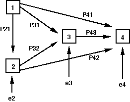
Consider the Model

Variable 1 is exogenous.
Variables 2,3 and 4 are endogenous.
The P_ij represent path coefficients from variable j to variable i.
The e_i represent errors or residuals for variable i.

Decomposition of correlations:

Each correlation can be decomposed into one or more of the following four types of effects:

Direct Effect (DE) - path coefficient from one variable to another, e.g., P₂₁.
Indirect Effect (IE) - sequence of paths through one or more intermediate variables, e.g., P₃₂P₂₁.
Unanalyzed Effect due to correlated causes (U) - correlation of variable with cause of the second, e.g., P₄₂P₃₁r₁₂.
Spurious Effect due to common cause (S) - variable that causes both first and second variable, e.g., P₄₁P₃₁.
Sum of Direct Effect (DE) and Indirect Effect (IE) = total causal part of the correlation between two variables.
Sum of Unanalyzed effect (U) and Spurious effect (S) = total noncausal part of the correlation between two variables.
Effects relating variables 1 and 2:

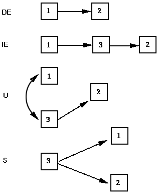
Path Tracing to Reproduce Correlations

Begin with any endogenous variable, i. Trace back along a path that comes from variable j. This is a direct path and the path coefficient P_ij represents a DE.
If other paths come to a variable from a third or more variables, k, trace all paths between i and j that involve k. Multiply the path coefficients creating compound paths.
While tracing paths do the following:
When all direct and compound path values have been calculated, add them together to obtain the reproduced correlation between i and j.

Example 1

With the following variables:

1 - SES

2 - IQ

3 - AM (achievement motivation)

4 - GPA

use http://www.philender.com/courses/data/ped788, clear

corr ses iq am gpa
(obs=300)

         |      ses       iq       am      gpa
---------+------------------------------------
     ses |   1.0000
      iq |   0.3000   1.0000
      am |   0.4100   0.1600   1.0000
     gpa |   0.3300   0.5700   0.5000   1.0000

regress iq ses, beta

  Source |       SS       df       MS                  Number of obs =     300
---------+------------------------------               F(  1,   298) =   29.47
   Model |  26.9099995     1  26.9099995               Prob > F      =  0.0000
Residual |  272.089997   298   .91305368               R-squared     =  0.0900
---------+------------------------------               Adj R-squared =  0.0869
   Total |  298.999996   299  .999999987               Root MSE      =  .95554

------------------------------------------------------------------------------
      iq |      Coef.   Std. Err.       t     P>|t|                       Beta
---------+--------------------------------------------------------------------
     ses |         .3   .0552602      5.429   0.000                         .3
   _cons |  -7.10e-09    .055168      0.000   1.000                          .
------------------------------------------------------------------------------

display sqrt(1-.09)
.9539392

regress am ses iq, beta

  Source |       SS       df       MS                  Number of obs =     300
---------+------------------------------               F(  2,   297) =   30.33
   Model |  50.7117145     2  25.3558572               Prob > F      =  0.0000
Residual |  248.288282   297  .835987481               R-squared     =  0.1696
---------+------------------------------               Adj R-squared =  0.1640
   Total |  298.999996   299  .999999988               Root MSE      =  .91432

------------------------------------------------------------------------------
      am |      Coef.   Std. Err.       t     P>|t|                       Beta
---------+--------------------------------------------------------------------
     ses |   .3978022   .0554298      7.177   0.000                   .3978022
      iq |   .0406593   .0554298      0.734   0.464                   .0406593
   _cons |  -8.73e-09   .0527885      0.000   1.000                          .
------------------------------------------------------------------------------

display sqrt(1-.1696)
.91126286

regress gpa am ses iq, beta

  Source |       SS       df       MS                  Number of obs =     300
---------+------------------------------               F(  3,   296) =   97.28
   Model |  148.445584     3  49.4818613               Prob > F      =  0.0000
Residual |  150.554414   296  .508629776               R-squared     =  0.4965
---------+------------------------------               Adj R-squared =  0.4914
   Total |  298.999998   299  .999999992               Root MSE      =  .71318

------------------------------------------------------------------------------
     gpa |      Coef.   Std. Err.       t     P>|t|                       Beta
---------+--------------------------------------------------------------------
      am |   .4161263   .0452609      9.194   0.000                   .4161263
     ses |   .0091893    .046835      0.196   0.845                   .0091893
      iq |    .500663   .0432751     11.569   0.000                    .500663
   _cons |   1.23e-09   .0411756      0.000   1.000                          .
------------------------------------------------------------------------------

display sqrt(1-.4965)
.70957734

Estimated path coefficients from multiple regression analyses:

P₂₁ = .300
P₃₁ = .398
P₃₂ = .041
P₄₁ = .009
P₄₂ = .501
P₄₃ = .416

Path Analysis: Example 1: Just Identified Model

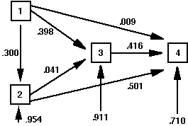
Compare actual and reproduced correlations: Model 1

To test whether the model fits the data, compare actual correlations to reproduced correlations based on paths in the model. We denote actual correlations by r and reproduced correlations by r*. The actual correlations are in brackets below.

r*₁₂	= P₂₁
	  DE
	= .300 [.300]
                
r*₁₃	= P₃₁ + P₃₂P₂₁
	  DE     IE
	= .398 + (.041)(.3) = .410 [.410]
                
r*₁₄	= P₄₁ + P₄₂P₂₁ + P₄₃P₃₁ + P₄₃P₃₂P₂₁
	  DE    IE      IE      IE       
	= .009+(.501)(.30)+(.416)(.398)+(.416)(.041)(.30) = .330 [.330]
	
r*₂₃	= P₃₁P₂₁ + P₃₂
	  S       DE
	= (.398)(.30) + .041 = .160 [.160]


r*₂₄	= P₄₁P₂₁ + P₄₂ + P₄₃P₃₁P₂₁ + P₄₃P₃₂
	  S        DE   S          IE
	= (.009)(.30)+(.501)+(.416)(.398)(.30)+(.416)(.041) = .570 [.570]
	
	
r*₃₄	= P₄₁P₃₁ + P₄₁P₂₁P₃₂ + P₄₂P₂₁P₃₁ + P₄₂P₃₂ + P₄₃
	  S       S          S		 S       DE
	= (.009)(.398)+(.009)(.30)(.041)+(.501)(.30)(.398)+(.501)(.041)+.416 = .500 [.500]

Note:

This is not a very interesting example because the reproduced and original correlations will be the same -- this model has all possible paths among the variables (i.e., no paths deleted).

Path Analysis: Model 2

A more interesting overidentified model

regress am ses, beta

  Source |       SS       df       MS                  Number of obs =     300
---------+------------------------------               F(  1,   298) =   60.22
   Model |  50.2619001     1  50.2619001               Prob > F      =  0.0000
Residual |  248.738096   298  .834691598               R-squared     =  0.1681
---------+------------------------------               Adj R-squared =  0.1653
   Total |  298.999996   299  .999999988               Root MSE      =  .91361

------------------------------------------------------------------------------
      am |      Coef.   Std. Err.       t     P>|t|                       Beta
---------+--------------------------------------------------------------------
     ses |        .41   .0528357      7.760   0.000                        .41
   _cons |  -9.02e-09   .0527476      0.000   1.000                          .
------------------------------------------------------------------------------

display sqrt(1-.1681)
.91208552

regress gpa iq am, beta

  Source |       SS       df       MS                  Number of obs =     300
---------+------------------------------               F(  2,   297) =  146.38
   Model |  148.426003     2  74.2130017               Prob > F      =  0.0000
Residual |  150.573994   297  .506983146               R-squared     =  0.4964
---------+------------------------------               Adj R-squared =  0.4930
   Total |  298.999998   299  .999999992               Root MSE      =  .71203

------------------------------------------------------------------------------
     gpa |      Coef.   Std. Err.       t     P>|t|                       Beta
---------+--------------------------------------------------------------------
      iq |   .5028736    .041715     12.055   0.000                   .5028736
      am |   .4195402    .041715     10.057   0.000                   .4195402
   _cons |   1.16e-09   .0411089      0.000   1.000                          .
------------------------------------------------------------------------------

display sqrt(1-.4964)
.7096478

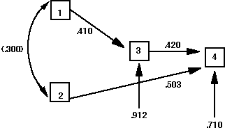
Reproduced correlations: Model 2

r*₁₂	= r₁₂ 
	  U
	= .30 [.30]

r*₁₃	= P₃₁     
	  DE        
	= .410  [.410]

r*₁₄	= P₄₂r₁₂ + P₄₃P₃₁  
	  U        IE         
	= (.503)(.30)+(.420)(.410) = .323 [.330]

r*₂₃	= P₃₁r₁₂     
	  U        
	= (.410)(.30) = .123  [.160]

r*₂₄	= P42 + P₄₃P₃₁r₁₂
	  DE    U                 
	= (.503)+(.420)(.410)(.30) = .555 [.570]

r*₃₄	= P₄₂P₃₁r₁₂ + P₄₃
	  U           DE
	= (.503)(.410)(.30)+(.420) = .482  [.50]

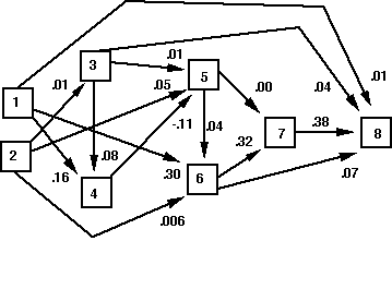
Terman Data Set

Variables:

1 - Parents education
2 - Father's occupation
3 - Parents attitude
4 - IQ
5 - Achievement
6 - Education level
7 - Occupation
8 - Income

Terman Model 1

Terman Model 2

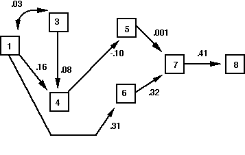
Reproduced Correlations: Terman Model 2

r*₁₄	= P₄₁ + P₄₃r₁₃  
	  DE    U

r*₁₅	= P₅₄P₄₁ + P₅₄P₄₃r₁₃ 
	  IE       U 

r*₁₆	= P₆₁  
	  DE

r*₁₇	= P₇₅P₅₄P₄₁ + P₇₅P₅₄P₄₃r₁₃ + P₇₆P₆₁ 
	  IE         U		   IE

r*₁₈	= P₈₇P₇₅P₅₄P₄₁ + P₈₇P₇₅P₅₄P_43r₁₃ + P₈₇P₇₆P₆₁
	  IE            U		 IE

r*₃₄	= P₄₁r₁₃ + P₄₃
	  U       DE

r*₃₅	= P₅₄P₄₁r₁₃ + P₅₄P₄₃
	  U          IE

r*₃₆	= P₆₁r₁₃
	  U

r*₃₇	= P₇₅P₅₄P₄₁r₁₃ + P₇₅P₅₄P₄₃ + P₇₆P₆₁r₁₃
	  U             IE	   U

r*₃₈	= P₈₇P₇₅P₅₄P₄₁r₁₃ + P₈₇P₇₅P₅₄P₄₃ + P₈₇P₇₆P₆₁r₁₃
	  U                IE	         U

r*₄₅	= P₅₄
	  DE

r*₄₆	= P₆₁P₄₁ + P₆₁P₄₃r₁₃
	  S        U
	  
r*₄₇	= P₇₅P₅₄ + P₇₆P₆₁P₄₁ + P₇₆P₆₁P₄₃r₁₃
	  IE       S	      U
	  
r*₄₈	= P₈₇P₇₅P₅₄ + P₈₇P₇₆P₆₁P₄₁ + P₈₇P₇₆P₆₁P₄₃r₁₃
	  IE          S	           U

r*₅₆	= P₆₁P₅₄P₄₁ + P₆₁P₅₄P₄₃r₁₃
	  S          U
	  
r*₅₇	= P₇₅ + P₇₆P₆₁P₅₄P₄₁ + P₇₆P₆₁P₅₄P₄₃r₁₃
	  DE    S	      U
	  
r*₅₈	= P₈₇P₇₅ + P₈₇P₇₆P₆₁P₅₄P₄₁ + P₈₇P₇₆P₆₁P₅₄P₄₃r₁₃
	  IE      S	           U
	  
r*₆₇	= P₇₅P₆₁P₅₄P₄₁ + P₇₅P₆₁P₅₄P₄₃r₁₃ + P₇₆
	  S             U	         DE
	  
r*₆₈	= P₈₇P₇₅P₆₁P₅₄P₄₁ + P₈₇P₇₅P₆₁P₅₄P₄₃r₁₃ + P₈₇P₇₆
	  S                U	              IE
	  
r*₇₈	= P₈₇
	  DE

Reproduced and actual correlations: Terman Model 2

r*₁₃  =  .03   [ .03]
r*₁₄  =  .16   [ .16]	
r*₁₅  = -.016  [ .07]  possible mismatch
r*₁₆  =  .31   [ .31]
r*₁₇  =  .10   [ .08]
r*₁₈  =  .04   [ .06]
r*₃₄  =  .08   [ .08]
r*₃₅  = -.008  [.003]		 
r*₃₆  =  .01   [ .14]  mismatch
r*₃₇  =  .003  [ .09]
r*₃₈  =  .001  [ .08]
r*₄₅  = -.10   [-.10]
r*₄₆  =  .05   [ .10]
r*₄₇  =  .02   [ .08]  possible mismatch
r*₄₈  =  .008  [ .09]  possible mismatch
r*₅₆  = -.005  [ .06]  possible mismatch
r*₅₇  = -.001  [ .02]
r*₅₈  =  .04   [-.01]
r*₆₇  =  .32   [ .32]
r*₆₈  =  .13   [ .20]  possible mismatch
r*₇₈  =  .41   [ .41]

Terman Model 3

EstimatedEquations: Terman Model 3

z'₆ = P₆₁ z₁
z'₇ = P₇₆ z₆
z'₈ = P₈₇ z₇

Reproduced and actual correlations: Terman Model 3

r*₁₆	= P₆₁ 
	  DE
	= .31 [.31]

r*₁₇	= P₇₆ p₆₁    
	  IE        
	= (.32)(.31) = .10  [.08]

r*₁₈	= P₈₇ P₇₆ P₆₁   
	  IE                         
	= (.41)(.32)(.31) = .04  [.06]

r*₆₇	= P₇₆     
	  DE        
	= .32  [.32]

r*₆₈	= P₈₇ P₇₆            
	  IE                              
	= (.41)(.32)  = .13  [.20]  (possible mismatch)

r*₇₈	= P₈₇  
	  DE      
	= .41 [.41]

Example Using Stata

We will use the hsbdemo dataset. For purposes of this example ses will be treated as continuous even thought it is categorical. In this example, ses and female will be exogenous while read and write will be endogenous. Here is our just identified model.


use http://www.philender.com/courses/data/hsbdemo, clear

corr ses female read write

(obs=200)

         |      ses   female     read    write
---------+------------------------------------
     ses |   1.0000
  female |  -0.1250   1.0000
    read |   0.2933  -0.0531   1.0000
   write |   0.2075   0.2565   0.5968   1.0000


regress read ses female, beta

  Source |       SS       df       MS                  Number of obs =     200
---------+------------------------------               F(  2,   197) =    9.30
   Model |  1805.58553     2  902.792765               Prob > F      =  0.0001
Residual |  19113.8345   197  97.0245405               R-squared     =  0.0863
---------+------------------------------               Adj R-squared =  0.0770
   Total |    20919.42   199  105.122714               Root MSE      =  9.8501

------------------------------------------------------------------------------
    read |      Coef.   Std. Err.       t     P>|t|                       Beta
---------+--------------------------------------------------------------------
     ses |   4.122699   .9716753      4.243   0.000                   .2912371
  female |  -.3425006    1.40975     -0.243   0.808                  -.0166765
   _cons |    43.94452   2.333705    18.83    0.000                          .
------------------------------------------------------------------------------

display sqrt(1 - .08632)

.9558661

regress write read ses female, beta

  Source |       SS       df       MS                  Number of obs =     200
---------+------------------------------               F(  3,   196) =   52.17
   Model |  7937.69723     3  2645.89908               Prob > F      =  0.0000
Residual |  9941.17777   196  50.7202947               R-squared     =  0.4440
---------+------------------------------               Adj R-squared =  0.4355
   Total |   17878.875   199   89.843593               Root MSE      =  7.1218

------------------------------------------------------------------------------
   write |      Coef.   Std. Err.       t     P>|t|                       Beta
---------+--------------------------------------------------------------------
    read |   .5470064    .051513     10.619   0.000                    .591694
     ses |   .9296443   .7339381      1.267   0.207                   .0710373
  female |   5.634919    1.01943      5.528   0.000                   .2967813
   _cons |    19.2234    2.823373     6.81    0.000                          .
------------------------------------------------------------------------------

display sqrt(1 - .444)

.74565408

Let's say that you are kind of lazy and don't want to run three separate regressions and compute the error at each stage. Here is a convenience command that you can use if you have Stata 7.

A Shortcut

/* user written progran -- findit pathreg */

pathreg (read ses female)(write ses read female)


------------------------------------------------------------------------------
        read |      Coef.   Std. Err.      t    P>|t|                     Beta
-------------+----------------------------------------------------------------
         ses |   4.122699   .9716753     4.24   0.000                 .2912371
      female |  -.3425006    1.40975    -0.24   0.808                -.0166765
       _cons |   43.94452   2.333705    18.83   0.000                        .
------------------------------------------------------------------------------
                 n = 200  R2 = 0.0863  sqrt(1 - R2) = 0.9559

------------------------------------------------------------------------------
       write |      Coef.   Std. Err.      t    P>|t|                     Beta
-------------+----------------------------------------------------------------
         ses |   .9296443   .7339381     1.27   0.207                 .0710373
        read |   .5470064    .051513    10.62   0.000                  .591694
      female |   5.634919    1.01943     5.53   0.000                 .2967813
       _cons |    19.2234   2.823373     6.81   0.000                        .
------------------------------------------------------------------------------
                 n = 200  R2 = 0.4440  sqrt(1 - R2) = 0.7457

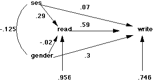
Reproducing Correlations

r*12 = r12
        U
     = -.125 [-.125]

r*13 = P31  + P32r12
        DE     U      
     = .29 +  (-.02)(-.125) = .29 [.29]

r*14 = P41  + P42r12      + P43P31 
        DE       U            IE       
     =  .07 + (.3)(-.125) + (.59)(.29) = .20 [.21]

r*23 = P32  + P31r12     
        DE      U        
     = -.02 + (.29)(-.125) = -.06  [-.05]

r*24 = P42 + P43P32    + P43P31r12       + P41r12
        DE     IE            U                U                
     =  .3 +(.59)(-.02)+(.59)(.29)(-.125)+(.07)(-.125) = .26 [.26]

r*34 = P43 + P42P32   + P41P31   + P42r12P31      + P41r12P32
        DE      IE        IE           S                S
     = .59 +(.3)(-.02)+(.07)(.29)+(.3)(-.125)(.29)+(.07)(-.125)(-.02) = .59 [.6]

Overidentified Model

Now let's look at an overidentified model.

pathreg (read ses)(write read female)

------------------------------------------------------------------------------
        read |      Coef.   Std. Err.      t    P>|t|                     Beta
-------------+----------------------------------------------------------------
         ses |    4.15221   .9617596     4.32   0.000                 .2933218
       _cons |   43.69721   2.095003    20.86   0.000                        .
------------------------------------------------------------------------------
                 n = 200  R2 = 0.0860  sqrt(1 - R2) = 0.9560

------------------------------------------------------------------------------
       write |      Coef.   Std. Err.      t    P>|t|                     Beta
-------------+----------------------------------------------------------------
        read |   .5658869   .0493849    11.46   0.000                 .6121169
      female |   5.486894   1.014261     5.41   0.000                 .2889851
       _cons |   20.22837   2.713756     7.45   0.000                        .
------------------------------------------------------------------------------
                 n = 200  R2 = 0.4394  sqrt(1 - R2) = 0.7487

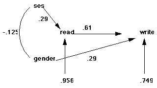
Reproducing Correlations

r*12 = r12
        U
     = -.125 [-.125]

r*13 = P31  
        DE        
     = .29  = .29 [.29]

r*14 = P42r12      +  P43P31 
          U             IE       
     = (.29)(-.125) + (.61)(.29) = .14 [.21]

r*23 = P31r12     
          U        
     = (.29)(-.125) = -.04  [-.05]

r*24 = P42 + P43P31r12 
        DE      U                         
     =  .29 +(.61)(.29)(-.125) = .28 [.26]

r*34 = P43 + P42r12P31    
        DE      S     
     = .61 + (.29)(-.125)(.29) = .6 [.6]

Linear Statistical Models Course

Phil Ender, 29Jan98