Descriptive Statistics and Exploratory Data Analysis

Of course, any data analysis would begin with descriptive statistics and exploratory data analysis. Included in these analyses would be distribution plots (histograms, stem plots, or kdensity plots).

Plot Dependent Variable vs Predicted Values

One visual check of the goodness-of-fit of the model is to plot the values of the dependent variable versus the predicted values. When there is perfect prediction the plot will be a diagonal line.

Residual Analysis

Residuals are the difference between the observed score and the predicted score.

Residuals come in three varieties:

1. Raw Residuals: The difference between the raw observed score and the predicted score, as given in the formula above. Often denoted e or resid.
2. Standardized Residuals: These are the raw residuals divided by the standard error of estimate. Can be denoted rstan or zresid.
3. Studentized Residuals: These are raw residuals divided by the standard error of the residual with that case deleted. These are sometimes called studentized deleted residuals or studentized jackknifed residuals. Can be denoted rstu.

Outliers are cases with large residuals.

• Look for studentized residuals greater than 2.5 in absolute value but don't become overly alarmed until residuals are greater than 3 or 4.
• Indicates a peculiarity -- data point is not typical of the rest of the data.
• These points should be examined carefully to try to find out why they are there. Perhaps there was an error in data entry or subjects did not understand instructions, etc.
• It is possible that observations with large residuals may have little effect on the estimation of b.
• What to do?
  • Automatic rejection -- not wise.
  • Possible data entry error -- correct error or delete case.
  • May be a "real" data point.

Plotting Residuals

• Plot shape of residuals (histogram, kdensity, normal probability).
• Plot of residuals by case (index plot).
• Plot of residuals in time sequence (if applicable).
• Plot of residual vs predicted, aka, residual vs fitted.
• Plot of residual vs each predictor variable.

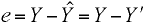
In General: Residual Plots

• You should get the impression of a horizontal band with points that vary at random.
• There should be no relation between residuals and predicted (fitted) score.

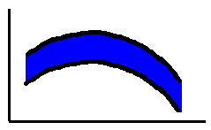
The picture should look something like this-

DV vs Predictors

• Plot DV vs IVs to check on linearity and association.

Overall Plot of Residuals

• Histogram
• Stem plot
• Normal probability plot

Index Plot -- Plot of Residuals by Case

• If sample is too large, list only cases with residuals greater than ±2.0.

Time Sequence Plot

• You should get impression of a horizontal band with points that vary at random.

1. Watch out for situations in which variance increases with time; try Weighted Least Squares (W.L.S.)

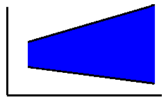
2. This pattern could indicate that a linear term is missing from the model.

3. This pattern could indicate that both a linear and a quadratic term in time are missing from the model.

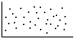
Plot Residuals versus Predicted (Fitted) Scores

• You should get the impression of a horizontal band with points that vary at random.
• There should be no relation between residuals and predicted scores.
• Square root of the absolute value of the residuals vesus fitted is good for checking for heterogeneity of vaiance.

1. Watch out for situations in which variance is not constant as assumed (may need W.L.S. or a transformation of Y).

2. This pattern could indicate that a variable is missing from the model (Also caused by wrongly omitting intercept term in model).

3. An additional term is needed in the model, the square of a variable or an interaction (again maybe transformation of Y).

Residual Plot versus Predictors

• You should get the impression of a horizontal band with points that vary at random.
• There should be no relation between residuals and IVs.
• Take care in inferring heteogeneity.

1. May need W.L.S. or a transformation of Y.

2. Perhaps errors in calculation?.

3. Need an additional term in X (X²) or transformation of Y..

Leverage

• An observation can be an outlier in another way besides having Y and Y' be far apart. The independent variable, x, can be far from the center of mass of the other x's.
• Leverage is a measure of how far an independent variable, X, deviates from its mean, Xbar.
• These points can have a large effect on the estimation of b.
• Such points are said to have high leverage.

Influence

• The fact that certain observations have greater influence on regression estimates than other.
• According to Belsley, Kuh & Welsch (1980), an infulential observations is "one which, either individually or together with several other observations, has demonstrably larger impact on the calculated values of various estimates (coefficients, standard errors, t-values, etc.) than is the case for most of the other observations."
• Consider influence to be the product of leverage and outlierness.

• Leverage (h) -- Sometimes called hat because it uses the diagonal elements of the hat matrix.
• Cook's distance (d) -- Combines information about both residuals and leverage.
• DFBETA -- Measures influence by comparing the b with the case included and excluded. A separate dfbeta can be computed for each predictor variable.

Measure	Value
leverage (h)	> (2k + 2)/n
rstu	> 2.5
cooksd (d)	> 4/n
|dfbeta|	> 2/sqrt(n)

Other Diagnostic Tests

regress gpa grev greq



  Source |       SS       df       MS                  Number of obs =      30
---------+------------------------------               F(  2,    27) =   12.73
   Model |  5.06332584     2  2.53166292               Prob > F      =  0.0001
Residual |  5.37134081    27  .198938548               R-squared     =  0.4852
---------+------------------------------               Adj R-squared =  0.4471
   Total |  10.4346666    29  .359816091               Root MSE      =  .44603

------------------------------------------------------------------------------
     gpa |      Coef.   Std. Err.       t     P>|t|       [95% Conf. Interval]
---------+--------------------------------------------------------------------
    grev |   .0027326   .0011288      2.421   0.022       .0004166    .0050487
    greq |   .0053559   .0019278      2.778   0.010       .0014003    .0093114
   _cons |  -1.286698   .9765207     -1.318   0.199      -3.290353    .7169566
------------------------------------------------------------------------------

Link test looks for one type of specification error.

linktest

  Source |       SS       df       MS                  Number of obs =      30
---------+------------------------------               F(  2,    27) =   13.50
   Model |  5.21793375     2  2.60896687               Prob > F      =  0.0001
Residual |   5.2167329    27  .193212329               R-squared     =  0.5001
---------+------------------------------               Adj R-squared =  0.4630
   Total |  10.4346666    29  .359816091               Root MSE      =  .43956

------------------------------------------------------------------------------
     gpa |      Coef.   Std. Err.       t     P>|t|       [95% Conf. Interval]
---------+--------------------------------------------------------------------
    _hat |  -2.744288   4.190284     -0.655   0.518      -11.34204    5.853464
  _hatsq |   .5622472   .6285344      0.895   0.379      -.7273988    1.851893
   _cons |    6.13873    6.89339      0.891   0.381      -8.005337     20.2828
------------------------------------------------------------------------------

ovtest

Ramsey RESET test using powers of the fitted values of gpa
       Ho:  model has no omitted variables
                  F(3, 24) =      1.20
                  Prob > F =      0.3307

hettest

Cook-Weisberg test for heteroscedasticity using fitted values of gpa
     Ho: Constant variance
         chi2(1)      =      0.03
         Prob > chi2  =      0.8686

whitetst   /* Downloaded from Stata (STB 55, sg137) via the Internet */

White's general test statistic :  10.10781  Chi-sq( 5)  P-value =  .0722