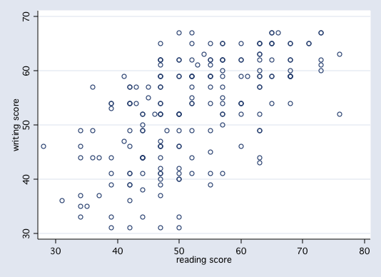
Let's consider two variables from the hsb2 dataset, write and read. In this example we will consider write to be our response variable and read to be our predictor variable, i.e., we want to be able to predict write from knowledge of read. Here is a scatter plot of the two variables.
    Variable |       Obs        Mean    Std. Dev.       Min        Max
-------------+--------------------------------------------------------
       write |        27    50.62963    9.245157         31         65


  3* | 1
  3. | 79
  4* | 01124
  4. | 6667
  5* | 22244
  5. | 77999
  6* | 1222
  6. | 5
We can do this for each of the values of read. Here is the frequency distribution and mean
value of write for each value of read.
    read |         N      mean write
---------+--------------------------
      28 |         1        46.00
      31 |         1        36.00
      34 |         6        40.67
      35 |         1        35.00
      36 |         3        50.00
      37 |         2        40.50
      39 |         8        43.63
      41 |         2        53.00
      42 |        13        46.00
      43 |         2        55.50
      44 |        13        44.92
      45 |         2        56.00
      46 |         1        52.00
      47 |        27        50.63
      48 |         1        49.00
      50 |        18        49.17
      52 |        14        56.00
      53 |         1        61.00
      54 |         1        63.00
      55 |        13        54.77
      57 |        14        56.86
      60 |         9        56.44
      61 |         1        59.00
      63 |        16        57.00
      65 |         9        62.56
      66 |         1        67.00
      68 |        11        60.27
      71 |         2        65.00
      73 |         5        63.40
      76 |         2        57.50
---------+--------------------------
   Total |       200        52.78
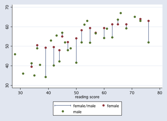
As you can see, some values of of read have only one value of write.
The distribution of write for each value of read is known as the conditional
distribution of write. The means are the conditional means, i.e., the means of
write conditioned on read.
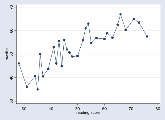
We can plot these conditional means versus read.
These means are the conditional means, i.e., the means of write conditioned on read.
We can plot these means versus read.
In linear regression we try to explain the change in the conditional mean of the response variable as a linear function of the predictor plus random error, i.e., Y = f(X) + e. We can plot this linear function as a straight line thusly,
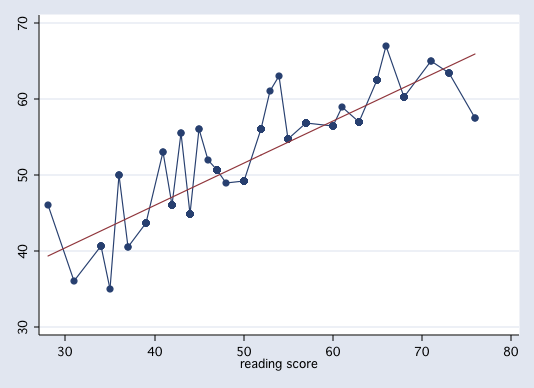
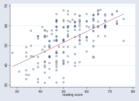
As was stated earlier the function f(X) is a linear function that defines a straight line. Any straight line can be completely determined by two parameters, the slope (b1) and the intercept (b0). For our example, b0 = 23.96 andb1 = 0.55, i.e., predicted write = f(x) = 23.96 + 0.55*read. In other words, the regression line is the line of all possible predicted values. Here is a table of all possible predicted scores, each of which falls on the least squares regression line.
reading   |    predicted
score     |    score
----------+-------------
       28 |    39.4072
       31 |    41.0623
       34 |    42.7174
       35 |    43.2691
       36 |    43.8208
       37 |    44.3725
       39 |    45.4759
       41 |    46.5794
       42 |    47.1311
       43 |    47.6828
       44 |    48.2345
       45 |    48.7862
       46 |    49.3379
       47 |    49.8896
       48 |    50.4413
       50 |    51.5447
       52 |    52.6481
       53 |    53.1998
       54 |    53.7515
       55 |    54.3032
       57 |    55.4066
       60 |    57.0617
       61 |    57.6135
       63 |    58.7169
       65 |    59.8203
       66 |    60.3720
       68 |    61.4754
       71 |    63.1305
       73 |    64.2339
       76 |    65.8890
Here are the results of running a regression of write on read.
------------------------------------------------------------------------------
       write |      Coef.   Std. Err.      t    P>|t|     [95% Conf. Interval]
-------------+----------------------------------------------------------------
        read |   .5517051   .0527178    10.47   0.000     .4477445    .6556656
       _cons |   23.95944   2.805744     8.54   0.000     18.42647    29.49242
------------------------------------------------------------------------------
And here are the results of running a regression of conditional means of write on read.
------------------------------------------------------------------------------
  mean write |      Coef.   Std. Err.      t    P>|t|     [95% Conf. Interval]
-------------+----------------------------------------------------------------
        read |   .5517051   .0196244    28.11   0.000     .5130053    .5904048
       _cons |   23.95944    1.04445    22.94   0.000     21.89977    26.01912
------------------------------------------------------------------------------
Note that the regression slopes and intercepts are the same in both models but that the
standard errors are different. The standard errors in the first model are the correct ones.