Linear Statistical Models
Robust Anova
Updated for Stata 11
When data do not completely meet the assumptions underlying the analysis of variance and/or
when there are outliers or influential data points robust anova procedures can be used.
The most basic robust procedures are to analyze the data using regression with robust
standard errors or to use the robust regression command rreg. Regress with the
robust option is more appropriate designs with heterogeneity of variance. The rreg
command is less useful except in situations with extreme outliers, although there may be other
ways of dealing with these kinds of outliers.
Of course, it is necessary to correctly code each of the categorical variables to use the
regression approach.
One-Factor Designs
In addition to robust regression techniques, the fstar and wtest commands
can be use with one-factor designs. Both fstar and wtest are more robust to
heteroscedasticity that regular one-way anova.
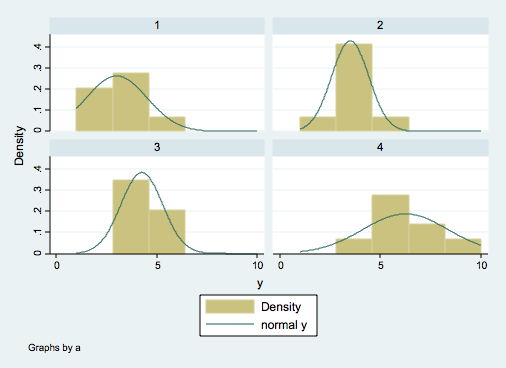
Consider an example using write as the response variable and prog as the categorical
variable.
use http://www.philender.com/courses/data/cr4new, clear

tabstat y, by(a) stat(n mean sd)

Summary for variables: y
     by categories of: a

       a |         N      mean        sd
---------+------------------------------
       1 |         8         3  1.511858
       2 |         8       3.5  .9258201
       3 |         8      4.25  1.035098
       4 |         8      6.25   2.12132
---------+------------------------------
   Total |        32      4.25  1.883716
----------------------------------------

histogram y, by(a) normal


anova y a

                           Number of obs =      32     R-squared     =  0.4455
                           Root MSE      =   1.476     Adj R-squared =  0.3860

                  Source |  Partial SS    df       MS           F     Prob > F
              -----------+----------------------------------------------------
                   Model |       49.00     3  16.3333333       7.50     0.0008
                         |
                       a |       49.00     3  16.3333333       7.50     0.0008
                         |
                Residual |       61.00    28  2.17857143
              -----------+----------------------------------------------------
                   Total |      110.00    31   3.5483871

regress y i.a


      Source |       SS       df       MS              Number of obs =      32
-------------+------------------------------           F(  3,    28) =    7.50
       Model |          49     3  16.3333333           Prob > F      =  0.0008
    Residual |          61    28  2.17857143           R-squared     =  0.4455
-------------+------------------------------           Adj R-squared =  0.3860
       Total |         110    31   3.5483871           Root MSE      =   1.476

------------------------------------------------------------------------------
           y |      Coef.   Std. Err.      t    P>|t|     [95% Conf. Interval]
-------------+----------------------------------------------------------------
           a |
          2  |         .5   .7379992     0.68   0.504    -1.011723    2.011723
          3  |       1.25   .7379992     1.69   0.101    -.2617229    2.761723
          4  |       3.25   .7379992     4.40   0.000     1.738277    4.761723
             |
       _cons |          3   .5218443     5.75   0.000      1.93105     4.06895
------------------------------------------------------------------------------

testparm i.a

 ( 1)  2.a = 0
 ( 2)  3.a = 0
 ( 3)  4.a = 0

       F(  3,    28) =    7.50
            Prob > F =    0.0008

regress y i.a, vce(robust)  /* useful with heterogeneity */


Linear regression                                      Number of obs =      32
                                                       F(  3,    28) =    5.02
                                                       Prob > F      =  0.0066
                                                       R-squared     =  0.4455
                                                       Root MSE      =   1.476

------------------------------------------------------------------------------
             |               Robust
           y |      Coef.   Std. Err.      t    P>|t|     [95% Conf. Interval]
-------------+----------------------------------------------------------------
           a |
          2  |         .5   .6267832     0.80   0.432    -.7839071    1.783907
          3  |       1.25   .6477985     1.93   0.064     -.076955    2.576955
          4  |       3.25   .9209855     3.53   0.001     1.363447    5.136553
             |
       _cons |          3   .5345225     5.61   0.000      1.90508     4.09492
------------------------------------------------------------------------------

testparm i.a

 ( 1)  2.a = 0
 ( 2)  3.a = 0
 ( 3)  4.a = 0

       F(  3,    28) =    5.02
            Prob > F =    0.0066

rreg y i.a   /* useful wirh outliers */

   Huber iteration 1:  maximum difference in weights = .53333333
   Huber iteration 2:  maximum difference in weights = .11280178
   Huber iteration 3:  maximum difference in weights = .02450832
Biweight iteration 4:  maximum difference in weights = .14902125
Biweight iteration 5:  maximum difference in weights = .02171319
Biweight iteration 6:  maximum difference in weights = .00926737

Robust regression                                      Number of obs =      32
                                                       F(  3,    28) =    7.51
                                                       Prob > F      =  0.0008

------------------------------------------------------------------------------
           y |      Coef.   Std. Err.      t    P>|t|     [95% Conf. Interval]
-------------+----------------------------------------------------------------
           a |
          2  |   .6744035   .7076641     0.95   0.349    -.7751807    2.123988
          3  |   1.404021   .7076641     1.98   0.057    -.0455634    2.853605
          4  |   3.183657   .7076641     4.50   0.000     1.734072    4.633241
             |
       _cons |   2.825597   .5003941     5.65   0.000     1.800586    3.850607
------------------------------------------------------------------------------

testparm i.a

 ( 1)  2.a = 0
 ( 2)  3.a = 0
 ( 3)  4.a = 0

       F(  3,    28) =    7.51
            Prob > F =    0.0008

fstar y a  /*  available from ATS via the Internet  */

----------------------------------------------------------------------
Dependent Variable is y and Independent Variable is a
Fstar(  3,  19.43) =   7.497, p= 0.0016
----------------------------------------------------------------------

wtest y a  /*  available from ATS via the Internet  */

----------------------------------------------------------------------
Dependent Variable is y and Independent Variable is a
WStat(  3,  15.06) =   4.612, p= 0.0176
----------------------------------------------------------------------
anova y a
Number of obs = 32 R-squared = 0.4455
Root MSE = 1.476 Adj R-squared = 0.3860
Source | Partial SS df MS F Prob > F
-----------+----------------------------------------------------
Model | 49.00 3 16.3333333 7.50 0.0008
|
a | 49.00 3 16.3333333 7.50 0.0008
|
Residual | 61.00 28 2.17857143
-----------+----------------------------------------------------
Total | 110.00 31 3.5483871
regress y i.a
Source | SS df MS Number of obs = 32
-------------+------------------------------ F( 3, 28) = 7.50
Model | 49 3 16.3333333 Prob > F = 0.0008
Residual | 61 28 2.17857143 R-squared = 0.4455
-------------+------------------------------ Adj R-squared = 0.3860
Total | 110 31 3.5483871 Root MSE = 1.476
------------------------------------------------------------------------------
y | Coef. Std. Err. t P>|t| [95% Conf. Interval]
-------------+----------------------------------------------------------------
a |
2 | .5 .7379992 0.68 0.504 -1.011723 2.011723
3 | 1.25 .7379992 1.69 0.101 -.2617229 2.761723
4 | 3.25 .7379992 4.40 0.000 1.738277 4.761723
|
_cons | 3 .5218443 5.75 0.000 1.93105 4.06895
------------------------------------------------------------------------------
testparm i.a
( 1) 2.a = 0
( 2) 3.a = 0
( 3) 4.a = 0
F( 3, 28) = 7.50
Prob > F = 0.0008
regress y i.a, vce(robust) /* useful with heterogeneity */
Linear regression Number of obs = 32
F( 3, 28) = 5.02
Prob > F = 0.0066
R-squared = 0.4455
Root MSE = 1.476
------------------------------------------------------------------------------
| Robust
y | Coef. Std. Err. t P>|t| [95% Conf. Interval]
-------------+----------------------------------------------------------------
a |
2 | .5 .6267832 0.80 0.432 -.7839071 1.783907
3 | 1.25 .6477985 1.93 0.064 -.076955 2.576955
4 | 3.25 .9209855 3.53 0.001 1.363447 5.136553
|
_cons | 3 .5345225 5.61 0.000 1.90508 4.09492
------------------------------------------------------------------------------
testparm i.a
( 1) 2.a = 0
( 2) 3.a = 0
( 3) 4.a = 0
F( 3, 28) = 5.02
Prob > F = 0.0066
rreg y i.a /* useful wirh outliers */
Huber iteration 1: maximum difference in weights = .53333333
Huber iteration 2: maximum difference in weights = .11280178
Huber iteration 3: maximum difference in weights = .02450832
Biweight iteration 4: maximum difference in weights = .14902125
Biweight iteration 5: maximum difference in weights = .02171319
Biweight iteration 6: maximum difference in weights = .00926737
Robust regression Number of obs = 32
F( 3, 28) = 7.51
Prob > F = 0.0008
------------------------------------------------------------------------------
y | Coef. Std. Err. t P>|t| [95% Conf. Interval]
-------------+----------------------------------------------------------------
a |
2 | .6744035 .7076641 0.95 0.349 -.7751807 2.123988
3 | 1.404021 .7076641 1.98 0.057 -.0455634 2.853605
4 | 3.183657 .7076641 4.50 0.000 1.734072 4.633241
|
_cons | 2.825597 .5003941 5.65 0.000 1.800586 3.850607
------------------------------------------------------------------------------
testparm i.a
( 1) 2.a = 0
( 2) 3.a = 0
( 3) 4.a = 0
F( 3, 28) = 7.51
Prob > F = 0.0008
fstar y a /* available from ATS via the Internet */
----------------------------------------------------------------------
Dependent Variable is y and Independent Variable is a
Fstar( 3, 19.43) = 7.497, p= 0.0016
----------------------------------------------------------------------
wtest y a /* available from ATS via the Internet */
----------------------------------------------------------------------
Dependent Variable is y and Independent Variable is a
WStat( 3, 15.06) = 4.612, p= 0.0176
----------------------------------------------------------------------
Nonparametric Test
We can also try a nonparametric test, such as the Kruskal-Wallis test. The Kruskal-Wallis is
the nonparametric analog of the one-way anova.
kwallis y, by(a)

Test: Equality of populations (Kruskal-Wallis test)

       a          _Obs   _RankSum
       1             8      78.50
       2             8     104.00
       3             8     142.50
       4             8     203.00

chi-squared =    12.496 with 3 d.f.
probability =     0.0059

chi-squared with ties =    12.997 with 3 d.f.
probability =     0.0046
Bootstrap Standard Errors
regress y i.a, vce(bootstrap, reps(200))

(running regress on estimation sample)

Bootstrap replications (200)
----+--- 1 ---+--- 2 ---+--- 3 ---+--- 4 ---+--- 5
..................................................    50
..................................................   100
..................................................   150
..................................................   200

Linear regression                               Number of obs      =        32
                                                Replications       =       200
                                                Wald chi2(3)       =     16.01
                                                Prob > chi2        =    0.0011
                                                R-squared          =    0.4455
                                                Adj R-squared      =    0.3860
                                                Root MSE           =    1.4760

------------------------------------------------------------------------------
             |   Observed   Bootstrap                         Normal-based
           y |      Coef.   Std. Err.      z    P>|z|     [95% Conf. Interval]
-------------+----------------------------------------------------------------
           a |
          2  |         .5   .6219155     0.80   0.421    -.7189321    1.718932
          3  |       1.25   .6431964     1.94   0.052    -.0106417    2.510642
          4  |       3.25    .935627     3.47   0.001     1.416205    5.083795
             |
       _cons |          3   .5212292     5.76   0.000      1.97841     4.02159
------------------------------------------------------------------------------

testparm i.a


 ( 1)  2.a = 0
 ( 2)  3.a = 0
 ( 3)  4.a = 0

           chi2(  3) =   16.01
         Prob > chi2 =    0.0011
Least Absolute Deviation
Minimizes the absolute values of deviations from the median, which is why it is
often known as median regression. We will run the example using bootstrap
standard errors with 200 replications. bsqreg does not work with factor
variables so we will use the xi: prefix.
xi: bsqreg y i.a, reps(200)

i.a               _Ia_1-4             (naturally coded; _Ia_1 omitted)
(fitting base model)
(bootstrapping)

Median regression, bootstrap(200) SEs                Number of obs =        32
  Raw sum of deviations       44 (about 4)
  Min sum of deviations       32                     Pseudo R2     =    0.2727

------------------------------------------------------------------------------
           y |      Coef.   Std. Err.      t    P>|t|     [95% Conf. Interval]
-------------+----------------------------------------------------------------
       _Ia_2 |          1   .8026182     1.25   0.223    -.6440889    2.644089
       _Ia_3 |          1   .7716067     1.30   0.206    -.5805647    2.580565
       _Ia_4 |          3   1.075819     2.79   0.009     .7962843    5.203716
       _cons |          3     .62749     4.78   0.000     1.714645    4.285355
------------------------------------------------------------------------------

test _Ia_2 _Ia_3 _Ia_4

 ( 1)  _Ia_2 = 0
 ( 2)  _Ia_3 = 0
 ( 3)  _Ia_4 = 0

       F(  3,    28) =    2.59
            Prob > F =    0.0725
Permutation Tests
Permutation tests are based on Monte Carlo simulations and can be used to test the differences
among the levels of the independent variable.
For each repetition, the values of group variable are randomly permuted, the test statistic
is computed, and a count is kept whether this value
of the test statistic is more extreme than the observed test statistic.
Stata uses the permute command along with an ado program to perform permutation tests.
Here is an example of a program that can be used with one-factor designs. It can be placed
in the data directory and should be named panova1.ado.
 program define panova1
   version 8
   args dv grp
   anova `dv' `grp'
 end
Here is how it is used with cr4new.
permute a "panova1 y a" F=e(F), reps(1000)

command:      panova1 y a
statistic:    F          = e(F)
permute var:  a

Monte Carlo permutation statistics                Number of obs    =        32
                                                  Replications     =      1000

------------------------------------------------------------------------------
T            |     T(obs)       c       n   p=c/n   SE(p) [95% Conf. Interval]
-------------+----------------------------------------------------------------
F            |   7.497268       1    1000  0.0010  0.0010  .0000253   .0055589
------------------------------------------------------------------------------
Note:  confidence interval is with respect to p=c/n
Note:  c = #{|T| >= |T(obs)|}
Next we will modify the dataset so that the results are not significant and repeat the
permutation tests.
replace y=4 in 29/32

anova y a

                           Number of obs =      32     R-squared     =  0.2220
                           Root MSE      = 1.12401     Adj R-squared =  0.1386

                  Source |  Partial SS    df       MS           F     Prob > F
              -----------+----------------------------------------------------
                   Model |    10.09375     3  3.36458333       2.66     0.0673
                         |
                       a |    10.09375     3  3.36458333       2.66     0.0673
                         |
                Residual |      35.375    28  1.26339286
              -----------+----------------------------------------------------
                   Total |    45.46875    31  1.46673387

permute a "panova1 y a" F=e(F), reps(1000)

command:      panova1 y a
statistic:    F          = e(F)
permute var:  a

Monte Carlo permutation statistics                Number of obs    =        32
                                                  Replications     =      1000

------------------------------------------------------------------------------
T            |     T(obs)       c       n   p=c/n   SE(p) [95% Conf. Interval]
-------------+----------------------------------------------------------------
F            |   2.663133      78    1000  0.0780  0.0085  .0621412   .0963936
------------------------------------------------------------------------------
Note:  confidence interval is with respect to p=c/n
Note:  c = #{|T| >= |T(obs)|}
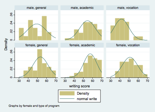
Two-Factor Designs
Consider a two-factor design using write as the response variable and female and
prog as the categorical independent variables.
use http://www.philender.com/courses/data/hsb2, clear

table female prog, contents(freq mean write sd write) row col

--------------------------------------------------
          |            type of program
   female |  general  academic  vocation     Total
----------+---------------------------------------
     male |       21        47        23        91
          | 49.14286  54.61702  41.82609  50.12088
          | 10.36478  8.656622  8.003705  10.30516
          |
   female |       24        58        27       109
          |    53.25  57.58621  50.96296  54.99083
          | 8.205248  7.115672  8.341193  8.133716
          |
    Total |       45       105        50       200
          | 51.33333  56.25714     46.76    52.775
          | 9.397776  7.943343  9.318754  9.478586
--------------------------------------------------

histogram write, by(female prog) start(30) width(5) normal

)

anova write female prog female#prog

                           Number of obs =     200     R-squared     =  0.2590
                           Root MSE      = 8.26386     Adj R-squared =  0.2399

                  Source |  Partial SS    df       MS           F     Prob > F
             ------------+----------------------------------------------------
                   Model |  4630.36091     5  926.072182      13.56     0.0000
                         |
                  female |  1261.85329     1  1261.85329      18.48     0.0000
                    prog |  3274.35082     2  1637.17541      23.97     0.0000
             female#prog |  325.958189     2  162.979094       2.39     0.0946
                         |
                Residual |  13248.5141   194  68.2913097
             ------------+----------------------------------------------------
                   Total |   17878.875   199   89.843593

regress write i.female##i.prog

      Source |       SS       df       MS              Number of obs =     200
-------------+------------------------------           F(  5,   194) =   13.56
       Model |  4630.36091     5  926.072182           Prob > F      =  0.0000
    Residual |  13248.5141   194  68.2913097           R-squared     =  0.2590
-------------+------------------------------           Adj R-squared =  0.2399
       Total |   17878.875   199   89.843593           Root MSE      =  8.2639

------------------------------------------------------------------------------
       write |      Coef.   Std. Err.      t    P>|t|     [95% Conf. Interval]
-------------+----------------------------------------------------------------
    1.female |   4.107143   2.469299     1.66   0.098    -.7629757    8.977261
             |
        prog |
          2  |   5.474164   2.169095     2.52   0.012     1.196128      9.7522
          3  |   -7.31677   2.494224    -2.93   0.004    -12.23605   -2.397493
             |
 female#prog |
        1 2  |  -1.137957   2.954299    -0.39   0.701    -6.964625     4.68871
        1 3  |   5.029733    3.40528     1.48   0.141    -1.686391    11.74586
             |
       _cons |   49.14286   1.803321    27.25   0.000     45.58623    52.69949
------------------------------------------------------------------------------

/* user written program -- findit anovalator */
/* test main effects and two-way interaction */

anovalator female prog, main 2way fratio

anovalator main-effect for female
chi2(1) = 18.477509   p-value = .00001719
scaled as F-ratio = 18.477509

anovalator main-effect for prog
chi2(2) = 47.946815   p-value = 3.877e-11
scaled as F-ratio = 23.973408

anovalator two-way interaction for female#prog
chi2(2) = 4.7730552   p-value = .09194841
scaled as F-ratio = 2.3865276

regress write i.female##i.prog, vce(robust)

Linear regression                                      Number of obs =     200
                                                       F(  5,   194) =   15.07
                                                       Prob > F      =  0.0000
                                                       R-squared     =  0.2590
                                                       Root MSE      =  8.2639

------------------------------------------------------------------------------
             |               Robust
       write |      Coef.   Std. Err.      t    P>|t|     [95% Conf. Interval]
-------------+----------------------------------------------------------------
    1.female |   4.107143   2.791816     1.47   0.143    -1.399066    9.613352
             |
        prog |
          2  |   5.474164   2.575164     2.13   0.035     .3952513    10.55308
          3  |   -7.31677   2.787331    -2.63   0.009    -12.81413   -1.819409
             |
 female#prog |
        1 2  |  -1.137957   3.207405    -0.35   0.723    -7.463818    5.187903
        1 3  |   5.029733    3.61924     1.39   0.166    -2.108377    12.16784
             |
       _cons |   49.14286   2.241144    21.93   0.000     44.72272    53.56299
------------------------------------------------------------------------------

/* robust tests of main effects and two-way interaction */

anovalator female prog, main 2way fratio


anovalator main-effect for female
chi2(1) = 16.859042   p-value = .00004026
scaled as F-ratio = 16.859042

anovalator main-effect for prog
chi2(2) = 49.702994   p-value = 1.611e-11
scaled as F-ratio = 24.851497

anovalator two-way interaction for female#prog
chi2(2) = 4.9516052   p-value = .08409547
scaled as F-ratio = 2.4758026

rreg write i.female##i.prog

   Huber iteration 1:  maximum difference in weights = .43221816
   Huber iteration 2:  maximum difference in weights = .0522718
   Huber iteration 3:  maximum difference in weights = .02118098
Biweight iteration 4:  maximum difference in weights = .15802072
Biweight iteration 5:  maximum difference in weights = .00897314

Robust regression                                      Number of obs =     200
                                                       F(  5,   194) =   14.17
                                                       Prob > F      =  0.0000

------------------------------------------------------------------------------
       write |      Coef.   Std. Err.      t    P>|t|     [95% Conf. Interval]
-------------+----------------------------------------------------------------
    1.female |   4.127819   2.561848     1.61   0.109    -.9248306    9.180468
             |
        prog |
          2  |   5.772446   2.250392     2.57   0.011      1.33407    10.21082
          3  |  -8.110425   2.587707    -3.13   0.002    -13.21408   -3.006774
             |
 female#prog |
        1 2  |  -1.307885   3.065025    -0.43   0.670    -7.352935    4.737164
        1 3  |   5.590185   3.532909     1.58   0.115    -1.377657    12.55803
             |
       _cons |   49.42263   1.870909    26.42   0.000      45.7327    53.11257
------------------------------------------------------------------------------

/* tests of main effects and two-way interaction following rreg */

anovalator female prog, main 2way fratio

anovalator main-effect for female
chi2(1) = 18.138295   p-value = .00002054
scaled as F-ratio = 18.138295

anovalator main-effect for prog
chi2(2) = 51.200604   p-value = 7.620e-12
scaled as F-ratio = 25.600302

anovalator two-way interaction for female#prog
chi2(2) = 5.5390472   p-value = .06269186
scaled as F-ratio = 2.7695236
)
anova write female prog female#prog
Number of obs = 200 R-squared = 0.2590
Root MSE = 8.26386 Adj R-squared = 0.2399
Source | Partial SS df MS F Prob > F
------------+----------------------------------------------------
Model | 4630.36091 5 926.072182 13.56 0.0000
|
female | 1261.85329 1 1261.85329 18.48 0.0000
prog | 3274.35082 2 1637.17541 23.97 0.0000
female#prog | 325.958189 2 162.979094 2.39 0.0946
|
Residual | 13248.5141 194 68.2913097
------------+----------------------------------------------------
Total | 17878.875 199 89.843593
regress write i.female##i.prog
Source | SS df MS Number of obs = 200
-------------+------------------------------ F( 5, 194) = 13.56
Model | 4630.36091 5 926.072182 Prob > F = 0.0000
Residual | 13248.5141 194 68.2913097 R-squared = 0.2590
-------------+------------------------------ Adj R-squared = 0.2399
Total | 17878.875 199 89.843593 Root MSE = 8.2639
------------------------------------------------------------------------------
write | Coef. Std. Err. t P>|t| [95% Conf. Interval]
-------------+----------------------------------------------------------------
1.female | 4.107143 2.469299 1.66 0.098 -.7629757 8.977261
|
prog |
2 | 5.474164 2.169095 2.52 0.012 1.196128 9.7522
3 | -7.31677 2.494224 -2.93 0.004 -12.23605 -2.397493
|
female#prog |
1 2 | -1.137957 2.954299 -0.39 0.701 -6.964625 4.68871
1 3 | 5.029733 3.40528 1.48 0.141 -1.686391 11.74586
|
_cons | 49.14286 1.803321 27.25 0.000 45.58623 52.69949
------------------------------------------------------------------------------
/* user written program -- findit anovalator */
/* test main effects and two-way interaction */
anovalator female prog, main 2way fratio
anovalator main-effect for female
chi2(1) = 18.477509 p-value = .00001719
scaled as F-ratio = 18.477509
anovalator main-effect for prog
chi2(2) = 47.946815 p-value = 3.877e-11
scaled as F-ratio = 23.973408
anovalator two-way interaction for female#prog
chi2(2) = 4.7730552 p-value = .09194841
scaled as F-ratio = 2.3865276
regress write i.female##i.prog, vce(robust)
Linear regression Number of obs = 200
F( 5, 194) = 15.07
Prob > F = 0.0000
R-squared = 0.2590
Root MSE = 8.2639
------------------------------------------------------------------------------
| Robust
write | Coef. Std. Err. t P>|t| [95% Conf. Interval]
-------------+----------------------------------------------------------------
1.female | 4.107143 2.791816 1.47 0.143 -1.399066 9.613352
|
prog |
2 | 5.474164 2.575164 2.13 0.035 .3952513 10.55308
3 | -7.31677 2.787331 -2.63 0.009 -12.81413 -1.819409
|
female#prog |
1 2 | -1.137957 3.207405 -0.35 0.723 -7.463818 5.187903
1 3 | 5.029733 3.61924 1.39 0.166 -2.108377 12.16784
|
_cons | 49.14286 2.241144 21.93 0.000 44.72272 53.56299
------------------------------------------------------------------------------
/* robust tests of main effects and two-way interaction */
anovalator female prog, main 2way fratio
anovalator main-effect for female
chi2(1) = 16.859042 p-value = .00004026
scaled as F-ratio = 16.859042
anovalator main-effect for prog
chi2(2) = 49.702994 p-value = 1.611e-11
scaled as F-ratio = 24.851497
anovalator two-way interaction for female#prog
chi2(2) = 4.9516052 p-value = .08409547
scaled as F-ratio = 2.4758026
rreg write i.female##i.prog
Huber iteration 1: maximum difference in weights = .43221816
Huber iteration 2: maximum difference in weights = .0522718
Huber iteration 3: maximum difference in weights = .02118098
Biweight iteration 4: maximum difference in weights = .15802072
Biweight iteration 5: maximum difference in weights = .00897314
Robust regression Number of obs = 200
F( 5, 194) = 14.17
Prob > F = 0.0000
------------------------------------------------------------------------------
write | Coef. Std. Err. t P>|t| [95% Conf. Interval]
-------------+----------------------------------------------------------------
1.female | 4.127819 2.561848 1.61 0.109 -.9248306 9.180468
|
prog |
2 | 5.772446 2.250392 2.57 0.011 1.33407 10.21082
3 | -8.110425 2.587707 -3.13 0.002 -13.21408 -3.006774
|
female#prog |
1 2 | -1.307885 3.065025 -0.43 0.670 -7.352935 4.737164
1 3 | 5.590185 3.532909 1.58 0.115 -1.377657 12.55803
|
_cons | 49.42263 1.870909 26.42 0.000 45.7327 53.11257
------------------------------------------------------------------------------
/* tests of main effects and two-way interaction following rreg */
anovalator female prog, main 2way fratio
anovalator main-effect for female
chi2(1) = 18.138295 p-value = .00002054
scaled as F-ratio = 18.138295
anovalator main-effect for prog
chi2(2) = 51.200604 p-value = 7.620e-12
scaled as F-ratio = 25.600302
anovalator two-way interaction for female#prog
chi2(2) = 5.5390472 p-value = .06269186
scaled as F-ratio = 2.7695236
Linear Statistical Models Course
Phil Ender, 17sep10, 15may06, 4apr06, 2apr02