Multi-way Factorial Designs

Linear Statistical Models: Regression

Multi-way Factorial Designs

Updataed for Stata 11

Linear Model for a 3 Factor Completely Randomized Factorial Design

Y_ijkl = μ + α_j + β_k + γ_l + αβ_jk + αγ_jl + βγ_kl + αβγ_jkl + ε_i(jkl)

where

μ is the overall population mean

α_j is the effect of level j

β_k is the effect of level k

γ_l is the effect of level l

αβ_jk is the joint effect of levels j & k

αγ_jl is the joint effect of levels j & l

βγ_kl is the joint effect of levels k & l

αβγ_jkl is the joint effect of levels j, k & l

&epsilon_i(jkl) is the experimental error nested within each group

A 3 Factor Completely Randomized Factorial Design

A

a1 a2 a3

C c1 B b1 27 22
45 28
76 33 31 37
52 45
86 66 55 62
76 85
104 126

b2 55 40
81 50
36 70 77 76
98 68
42 104 132 104
96 70
89 142

c2 B b1 61 39
76 60
46 59 61 71
82 92
103 105 140 122
99 92
68 101

b2 88 92
95 103
51 73 100 120
120 131
89 76 142 150
96 105
80 125

A

a1 a2 a3

C c1 B b1 S₁
n = 6 S₂
n = 6 S₃
n = 6

b2 S₄
n = 6 S₅
n = 6 S₆
n = 6

c2 B b1 S₇
n = 6 S₈
n = 6 S₉
n = 6

b2 S₁₀
n = 6 S₁₁
n = 6 S₁₂
n = 6

ANOVA Summary Table

Source SS df MS F
A Main effect 23630 2 11815 24.64
B Main effect 7667 1 7667 15.99
C Main effect 9730 1 9730 20.29
A*B Interaction   136 2    68 .14
A*C Interaction   752 2   376 .78
B*C Interaction    9 1     9 .02
A*B*C Interaction   224 2   112 .23
Within Cells 28769 60 479
Total 70917 71

Model for Orthogonal Coding

      A      B   C   A*B     A*C     B*C A*B*C
A B C X1 X2  X3  X4  X5  X6  X7  X8  X9  X10  X11
1 1 1  1  1   1   1   1   1   1   1   1    1   1
2 1 1 -1  1   1   1  -1   1  -1   1   1   -1   1
3 1 1  0 -2   1   1   0  -2   0  -2   1    0  -2
1 2 1  1  1  -1   1  -1  -1   1   1  -1   -1  -1
2 2 1 -1  1  -1   1   1  -1  -1   1  -1    1  -1
3 2 1  0 -2  -1   1   0   2   0  -2  -1    0   2
1 1 2  1  1   1  -1   1   1  -1  -1  -1   -1  -1
2 1 2 -1  1   1  -1  -1   1   1  -1  -1    1  -1
3 1 2  0 -2   1  -1   0  -2   0   2  -1    0   2
1 2 2  1  1  -1  -1  -1  -1  -1  -1   1    1   1
2 2 2 -1  1  -1  -1   1  -1   1  -1   1   -1   1
3 2 2  0 -2  -1  -1   0   2   0   2   1    0  -2

Stata Example

input y a b c x1 x2 x3 x4
 27 1 1 1   1  1  1  1
 22 1 1 1   1  1  1  1
 45 1 1 1   1  1  1  1
 18 1 1 1   1  1  1  1
 76 1 1 1   1  1  1  1
 33 1 1 1   1  1  1  1
 31 2 1 1  -1  1  1  1
 37 2 1 1  -1  1  1  1
 52 2 1 1  -1  1  1  1
 45 2 1 1  -1  1  1  1
 86 2 1 1  -1  1  1  1
 66 2 1 1  -1  1  1  1
 55 3 1 1   0 -2  1  1
 62 3 1 1   0 -2  1  1
 76 3 1 1   0 -2  1  1
 85 3 1 1   0 -2  1  1
104 3 1 1   0 -2  1  1
126 3 1 1   0 -2  1  1
 55 1 2 1   1  1 -1  1
 40 1 2 1   1  1 -1  1
 81 1 2 1   1  1 -1  1
 50 1 2 1   1  1 -1  1
 36 1 2 1   1  1 -1  1
 70 1 2 1   1  1 -1  1
 77 2 2 1  -1  1 -1  1
 76 2 2 1  -1  1 -1  1
 98 2 2 1  -1  1 -1  1
 68 2 2 1  -1  1 -1  1
 42 2 2 1  -1  1 -1  1
104 2 2 1  -1  1 -1  1
132 3 2 1   0 -2 -1  1
104 3 2 1   0 -2 -1  1
 96 3 2 1   0 -2 -1  1
 70 3 2 1   0 -2 -1  1
 89 3 2 1   0 -2 -1  1
142 3 2 1   0 -2 -1  1
 61 1 1 2   1  1  1 -1
 39 1 1 2   1  1  1 -1
 76 1 1 2   1  1  1 -1
 60 1 1 2   1  1  1 -1
 46 1 1 2   1  1  1 -1
 59 1 1 2   1  1  1 -1
 61 2 1 2  -1  1  1 -1
 71 2 1 2  -1  1  1 -1
 82 2 1 2  -1  1  1 -1
 92 2 1 2  -1  1  1 -1
103 2 1 2  -1  1  1 -1
105 2 1 2  -1  1  1 -1
140 3 1 2   0 -2  1 -1
122 3 1 2   0 -2  1 -1
 99 3 1 2   0 -2  1 -1
 92 3 1 2   0 -2  1 -1
 68 3 1 2   0 -2  1 -1
101 3 1 2   0 -2  1 -1
 88 1 2 2   1  1 -1 -1
 92 1 2 2   1  1 -1 -1
 95 1 2 2   1  1 -1 -1
103 1 2 2   1  1 -1 -1
 51 1 2 2   1  1 -1 -1
 73 1 2 2   1  1 -1 -1
100 2 2 2  -1  1 -1 -1
120 2 2 2  -1  1 -1 -1
120 2 2 2  -1  1 -1 -1
131 2 2 2  -1  1 -1 -1
 89 2 2 2  -1  1 -1 -1
 76 2 2 2  -1  1 -1 -1
142 3 2 2   0 -2 -1 -1
150 3 2 2   0 -2 -1 -1
 96 3 2 2   0 -2 -1 -1
105 3 2 2   0 -2 -1 -1
 80 3 2 2   0 -2 -1 -1
125 3 2 2   0 -2 -1 -1
end

generate x5=x1*x3
generate x6=x2*x3
generate x7=x1*x4
generate x8=x2*x4
generate x9=x3*x4
generate x10=x1*x3*x4
generate x11=x2*x3*x4

table a, cont(freq mean y sd y) by(b c) 

----------+-----------------------------------
b, c and  |
a         |      Freq.     mean(y)       sd(y)
----------+-----------------------------------
1         |
1         |
        1 |          6    36.83333    21.38613
        2 |          6    52.83333    20.31174
        3 |          6    84.66666    26.65083
----------+-----------------------------------
1         |
2         |
        1 |          6    56.83333    12.92156
        2 |          6    85.66666    17.61439
        3 |          6    103.6667    24.87301
----------+-----------------------------------
2         |
1         |
        1 |          6    55.33333    17.38582
        2 |          6        77.5    22.25084
        3 |          6       105.5    27.05365
----------+-----------------------------------
2         |
2         |
        1 |          6    83.66666    18.82197
        2 |          6         106    21.17546
        3 |          6    116.3333    27.31056
----------+-----------------------------------
	   
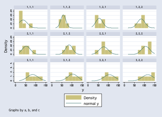
histogram y, by(a b c) normal 



anova y a b c a#b a#c b#c a#b#c
  
                           Number of obs =      72     R-squared     =  0.5943
                           Root MSE      = 21.8973     Adj R-squared =  0.5199

                  Source |  Partial SS    df       MS           F     Prob > F
              -----------+----------------------------------------------------
                   Model |  42147.8194    11  3831.61995       7.99     0.0000
                         |
                       a |  23630.0278     2  11815.0139      24.64     0.0000
                       b |  7667.34722     1  7667.34722      15.99     0.0002
                       c |    9730.125     1    9730.125      20.29     0.0000
                     a#b |  136.194444     2  68.0972222       0.14     0.8679
                     a#c |      751.75     2     375.875       0.78     0.4612
                     b#c |  8.68055556     1  8.68055556       0.02     0.8934
                   a#b#c |  223.694444     2  111.847222       0.23     0.7927
                         |
                Residual |     28769.5    60  479.491667   
              -----------+----------------------------------------------------
                   Total |  70917.3194    71  998.835485  
             
regress y x1 x2 x3 x4 x5 x6 x7 x8 x9 x10 x11

      Source |       SS       df       MS              Number of obs =      72
-------------+------------------------------           F( 11,    60) =    7.99
       Model |  42147.8194    11  3831.61995           Prob > F      =  0.0000
    Residual |     28769.5    60  479.491667           R-squared     =  0.5943
-------------+------------------------------           Adj R-squared =  0.5199
       Total |  70917.3194    71  998.835485           Root MSE      =  21.897

------------------------------------------------------------------------------
           y |      Coef.   Std. Err.      t    P>|t|     [95% Conf. Interval]
-------------+----------------------------------------------------------------
          x1 |  -11.16667   3.160603    -3.53   0.001    -17.48881    -4.84452
          x2 |  -11.06944   1.824775    -6.07   0.000    -14.71954   -7.419351
          x3 |  -10.31944   2.580621    -4.00   0.000    -15.48146   -5.157433
          x4 |    -11.625   2.580621    -4.50   0.000    -16.78701   -6.462989
          x5 |  -.0416667   3.160603    -0.01   0.990    -6.363813     6.28048
          x6 |  -.9722222   1.824775    -0.53   0.596    -4.622315    2.677871
          x7 |      1.625   3.160603     0.51   0.609    -4.697147    7.947147
          x8 |  -2.083333   1.824775    -1.14   0.258    -5.733426     1.56676
          x9 |  -.3472222   2.580621    -0.13   0.893    -5.509233    4.814789
         x10 |   1.583333   3.160603     0.50   0.618    -4.738813     7.90548
         x11 |   .8472222   1.824775     0.46   0.644    -2.802871    4.497315
       _cons |   80.40278   2.580621    31.16   0.000     75.24077    85.56479
------------------------------------------------------------------------------

test x1 x2

 ( 1)  x1 = 0.0
 ( 2)  x2 = 0.0

       F(  2,    60) =   24.64
            Prob > F =    0.0000

test x3

 ( 1)  x3 = 0.0

       F(  1,    60) =   15.99
            Prob > F =    0.0002            

test x4

 ( 1)  x4 = 0.0

       F(  1,    60) =   20.29
            Prob > F =    0.0000

test x5 x6

 ( 1)  x5 = 0.0
 ( 2)  x6 = 0.0

       F(  2,    60) =    0.14
            Prob > F =    0.8679                   

test x7 x8

 ( 1)  x7 = 0.0
 ( 2)  x8 = 0.0

       F(  2,    60) =    0.78
            Prob > F =    0.4612

test x9

 ( 1)  x9 = 0.0

       F(  1,    60) =    0.02
            Prob > F =    0.893

test x10 x11

 ( 1)  x10 = 0.0
 ( 2)  x11 = 0.0

       F(  2,    60) =    0.23
            Prob > F =    0.792

From Computer Example


regress y x1 x2 x3 x4 x5 x6 x7 x8 x9 x10 x11 /* m0 */
regress y x1 x2                              /* m1 */
regress y x3                                 /* m2 */
regress y x4                                 /* m3 */
regress y x5 x6                              /* m4 */
regress y x7 x8                              /* m5 */
regress y x9                                 /* m6 */
regress y x10 x11                            /* m7 */

Regression Results Summarized

Model: m0  R-squared     0.5943
Model: m1  R-squared     0.3332
Model: m2  R-squared     0.1081
Model: m3  R-squared     0.1372
Model: m4  R-squared     0.0019
Model: m5  R-squared     0.0106
Model: m6  R-squared     0.0001
Model: m7  R-squared     0.0032

F-ratios Using Regression

F-ratio for A*B*C interaction

F-ratio for A*B interaction

F-ratio for A*C interaction

F-ratio for B*C interaction

F-ratio for A main effect

F-ratio for B main effect

F-ratio for C main effect

Pooling Around

Let's try pooling the three way interaction. I'm not necessarily recommending pooling, but let's see what happens. Use this Stata code with the previous three factor dataset.

anova y a b c a#b a#c b#c

                           Number of obs =      72     R-squared     =  0.5912
                           Root MSE      = 21.6248     Adj R-squared =  0.5318

                  Source |  Partial SS    df       MS           F     Prob > F
              -----------+----------------------------------------------------
                   Model |   41924.125     9  4658.23611       9.96     0.0000
                         |
                       a |  23630.0278     2  11815.0139      25.27     0.0000
                       b |  7667.34722     1  7667.34722      16.40     0.0001
                       c |    9730.125     1    9730.125      20.81     0.0000
                     a#b |  136.194444     2  68.0972222       0.15     0.8648
                     a#c |      751.75     2     375.875       0.80     0.4522
                     b#c |  8.68055556     1  8.68055556       0.02     0.8921
                         |
                Residual |  28993.1944    62  467.632168   
              -----------+----------------------------------------------------
                   Total |  70917.3194    71  998.835485

More Pooling

Now let's try pooling all of the two way interactions. Use this Stata code with the previous three factor dataset.

anova y a b c

                      Number of obs =      72     R-squared     =  0.5785
                      Root MSE      = 21.1215     Adj R-squared =  0.5534

             Source |  Partial SS    df       MS           F     Prob > F
         -----------+----------------------------------------------------
              Model |    41027.50     4   10256.875      22.99     0.0000
                    |
                  a |  23630.0278     2  11815.0139      26.48     0.0000
                  b |  7667.34722     1  7667.34722      17.19     0.0001
                  c |    9730.125     1    9730.125      21.81     0.0000
                    |
           Residual |  29889.8194    67  446.116708   
         -----------+----------------------------------------------------
              Total |  70917.3194    71  998.835485

Consider a 3 Factor Random Effects Model

Expected Mean Squares

It is clear from inspection of the expected mean squares that there are no error terms for the A, B, & C Main Effects.

Quasi F-ratio

One solution is to use quasi F-ratios

For example for A main effect:

Compute denominator degrees of freedom as follows:

Use nearest integer value for df.

Combining the expected mean squares shows how this quasi F-ratio works

A problem with F' which leads to F''

A problem that can occur with the F' quasi F-ration is a negative denominator.

In that case use F'' as illustrated below on the A main effect:

With numerator degrees fo freedom computer as follows:

Use nearest integer value for df.

With denominator degrees fo freedom computer as follows:

Use nearest integer value for df.

How F'' Works

Numerator of F'':

Denominator of F'':

Linear Statistical Models Course

Phil Ender, 24sep10, 19apr06, 12Feb98

				A
				a1	a2	a3
C	c1	B	b1	27 22 45 28 76 33	31 37 52 45 86 66	55 62 76 85 104 126
	c1	B	b2	55 40 81 50 36 70	77 76 98 68 42 104	132 104 96 70 89 142
	c2	B	b1	61 39 76 60 46 59	61 71 82 92 103 105	140 122 99 92 68 101
	c2	B	b2	88 92 95 103 51 73	100 120 120 131 89 76	142 150 96 105 80 125

				A
				a1	a2	a3
C	c1	B	b1	S₁ n = 6	S₂ n = 6	S₃ n = 6
	c1	B	b2	S₄ n = 6	S₅ n = 6	S₆ n = 6
	c2	B	b1	S₇ n = 6	S₈ n = 6	S₉ n = 6
	c2	B	b2	S₁₀ n = 6	S₁₁ n = 6	S₁₂ n = 6

Source	SS	df	MS	F
A Main effect	23630	2	11815	24.64
B Main effect	7667	1	7667	15.99
C Main effect	9730	1	9730	20.29
A*B Interaction	136	2	68	.14
A*C Interaction	752	2	376	.78
B*C Interaction	9	1	9	.02
ABC Interaction	224	2	112	.23
Within Cells	28769	60	479
Total	70917	71