
Model for Orthogonal Coding
    A Main  B Main  A*B Interaction
A B X1 X2   X3 X4   X5 X6 X7 X8
1 1  1  1    1  1    1  1  1  1
1 2  1  1   -1  1   -1  1 -1  1
1 3  1  1    0 -2    0 -2  0 -2
2 1 -1  1    1  1   -1 -1  1  1
2 2 -1  1   -1  1    1 -1 -1  1
2 3 -1  1    0 -2    0  2  0 -2
3 1  0 -2    1  1    0  0 -2 -2
3 2  0 -2   -1  1    0  0  2 -2
3 3  0 -2    0 -2    0  0  0  4
Stata Computer Example
input a b y x1 x2 x3 x4
1 1 24 1 1 1 1
1 1 33 1 1 1 1
1 1 37 1 1 1 1
1 1 29 1 1 1 1
1 1 42 1 1 1 1
1 2 44 1 1 -1 1
1 2 36 1 1 -1 1
1 2 25 1 1 -1 1
1 2 27 1 1 -1 1
1 2 43 1 1 -1 1
1 3 38 1 1 0 -2
1 3 29 1 1 0 -2
1 3 28 1 1 0 -2
1 3 47 1 1 0 -2
1 3 48 1 1 0 -2
2 1 30 -1 1 1 1
2 1 21 -1 1 1 1
2 1 39 -1 1 1 1
2 1 26 -1 1 1 1
2 1 34 -1 1 1 1
2 2 35 -1 1 -1 1
2 2 40 -1 1 -1 1
2 2 27 -1 1 -1 1
2 2 31 -1 1 -1 1
2 2 22 -1 1 -1 1
2 3 26 -1 1 0 -2
2 3 27 -1 1 0 -2
2 3 36 -1 1 0 -2
2 3 46 -1 1 0 -2
2 3 45 -1 1 0 -2
3 1 21 0 -2 1 1
3 1 18 0 -2 1 1
3 1 10 0 -2 1 1
3 1 31 0 -2 1 1
3 1 20 0 -2 1 1
3 2 41 0 -2 -1 1
3 2 39 0 -2 -1 1
3 2 50 0 -2 -1 1
3 2 36 0 -2 -1 1
3 2 34 0 -2 -1 1
3 3 42 0 -2 0 -2
3 3 52 0 -2 0 -2
3 3 53 0 -2 0 -2
3 3 49 0 -2 0 -2
3 3 64 0 -2 0 -2
end
generate x5 = x1*x3
generate x6 = x1*x4
generate x7 = x2*x3
generate x8 = x2*x4
or
use http://www.gseis.ucla.edu/courses/data/crf33a, clear
table b,cont(freq mean y sd y) by(a)
----------+-----------------------------------
a and b | Freq. mean(y) sd(y)
----------+-----------------------------------
1 |
1 | 5 33 6.964194
2 | 5 35 8.803409
3 | 5 38 9.513149
----------+-----------------------------------
2 |
1 | 5 30 6.964194
2 | 5 31 6.964194
3 | 5 36 9.513149
----------+-----------------------------------
3 |
1 | 5 20 7.516648
2 | 5 40 6.204837
3 | 5 52 7.968688
----------+-----------------------------------
parcoord a b y /* available from Stata STB 29 */
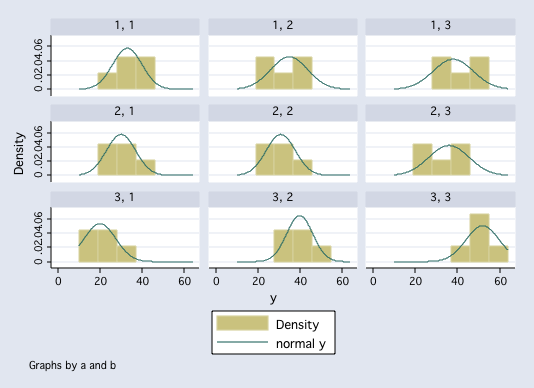
 histogram y, by(a b) normal
 anova y a b a*b
Number of obs = 45 R-squared = 0.5690
Root MSE = 7.90569 Adj R-squared = 0.4732
Source | Partial SS df MS F Prob > F
-----------+----------------------------------------------------
Model | 2970.00 8 371.25 5.94 0.0001
|
a | 190.00 2 95.00 1.52 0.2324
b | 1543.33333 2 771.666667 12.35 0.0001
a*b | 1236.66667 4 309.166667 4.95 0.0028
|
Residual | 2250.00 36 62.50
-----------+----------------------------------------------------
Total | 5220.00 44 118.636364
omega2 b
omega squared for b = 0.3352
effect size = 0.7101
omega2 a*b
omega squared for a*b = 0.2597
effect size = 0.5923
anova y a b a*b
Number of obs = 45 R-squared = 0.5690
Root MSE = 7.90569 Adj R-squared = 0.4732
Source | Partial SS df MS F Prob > F
-----------+----------------------------------------------------
Model | 2970.00 8 371.25 5.94 0.0001
|
a | 190.00 2 95.00 1.52 0.2324
b | 1543.33333 2 771.666667 12.35 0.0001
a*b | 1236.66667 4 309.166667 4.95 0.0028
|
Residual | 2250.00 36 62.50
-----------+----------------------------------------------------
Total | 5220.00 44 118.636364
omega2 b
omega squared for b = 0.3352
effect size = 0.7101
omega2 a*b
omega squared for a*b = 0.2597
effect size = 0.5923Plotting Cell Means
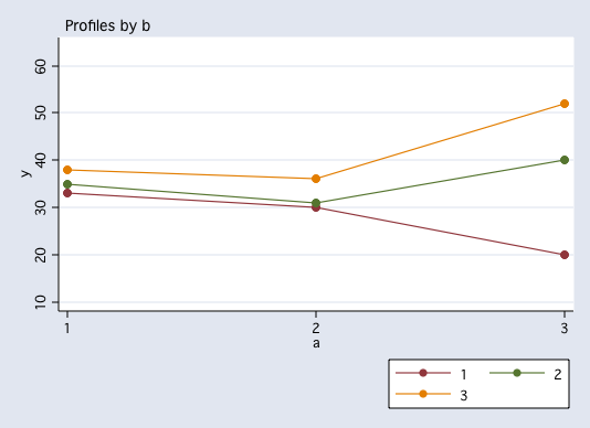
anovaplot b a, scatter(msym(none)) /* findit anovaplot */anovaplot a b, scatter(msym(none)) /* findit anovaplot */
Phil Ender, 12Feb98