CRF-pq -- Fixed Effects Model
Schematic with Example Data
IV B b1
b2 b3 A a1 24
33
37
29
42
44
36
25
27
43
38
29
28
47
48
a2 30
21
39
26
34
35
40
27
31
22
26
27
36
46
45
a3 21
18
10
31
20
41
39
50
36
34
42
52
53
49
64
Or in abbreviated form
IV B b1
b2 b3 A a1 S1
n=5
S2
n=5
S3
n=5
a2 S4
n=5
S5
n=5
S6
n=5
a3 S7
n=5
S8
n=5
S9
n=5
Where each Sj is an independent randomly assigned group of subjects.
Linear Model
Yijkl = μ + αj + βk + γl + αβjk + αγjl + βγkl + αβγjkl + εi(jkl)
where,
Yijk is the score for the ith observation in the
jkth treatment combination
μ is the overall population mean (grand mean)
αj is the effect of A treatment level j which is equal to
μj. - μ
βk is the effect of B treatment level k which is equal to
μ.k - μ
αβjk is the joint effect of treatment levels j and k
which is equal to
μjk - μj. -
μ.k + μ
εi(jk) is the error effect associated with Yijk
and is equal to Yijk - μ - αj
- βk - αβjk.
The error effect is a random variable that is
distributed NID(0,s2ε)
Further:
Σαj = 0 over j
Σβk = 0 over k
Σαβjk = 0 over j
Σαβjk = 0 over k
Hypotheses
Assumptions
1. The linear model reflects all sources of variation.
2. The experiment contains all the treatment levels of interest.
3. The εi(jk) are independent of each other.
4. The εi(jk) are normally distributed in the population.
5. The εi(jk) have equal variance in the population.
ANOVA Summary Table
| Source | SS | df | MS | F | p-value |
| A Main effect | 190.000 | 2 | 95.00 | 1.52 | .2324 |
| B Main effect | 1543.333 | 2 | 771.67 | 12.35 | .0001 |
| A*B Interaction | 1236.667 | 4 | 309.17 | 4.95 | .0028 |
| Within Cells | 2250.000 | 36 | 62.50 | ||
| Total | 5220.000 | 44 |
Fixed-Effects Expected Mean Squares
Cell Means & Standard Deviations
| b1 | b2 | b3 | |
| a1 | 33 6.96 | 35 8.80 | 38 9.51 |
| a2 | 30 6.96 | 31 6.96 | 36 9.51 |
| a3 | 20 7.52 | 40 6.20 | 52 7.97 |
egen cell=group(a b)

tablist cell a b, clean

    cell   a   b   Freq
       1   1   1      5
       2   1   2      5
       3   1   3      5
       4   2   1      5
       5   2   2      5
       6   2   3      5
       7   3   1      5
       8   3   2      5
       9   3   3      5

tabstat y, by(cell) stat(n mean sd var)

Summary for variables: y
     by categories of: cell (group(a b))

    cell |         N      mean        sd  variance
---------+----------------------------------------
       1 |         5        33  6.964194      48.5
       2 |         5        35  8.803408      77.5
       3 |         5        38  9.513149      90.5
       4 |         5        30  6.964194      48.5
       5 |         5        31  6.964194      48.5
       6 |         5        36  9.513149      90.5
       7 |         5        20  7.516648      56.5
       8 |         5        40  6.204837      38.5
       9 |         5        52  7.968689      63.5
---------+----------------------------------------
   Total |        45        35  10.89203  118.6364
--------------------------------------------------
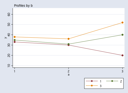
Graph of Cell Means
Strength of Association
In this example, variables A and B are fixed effects and the appropriate measure of association is the partial omega squared (see Kirk page 397).
For the CRF33 example:
If ω2 is negative set ω2 to equal zero.
Model for Orthogonal Coding
    A Main  B Main  A*B Interaction
A B X1 X2   X3 X4   X5 X6 X7 X8
1 1  1  1    1  1    1  1  1  1
1 2  1  1   -1  1   -1  1 -1  1
1 3  1  1    0 -2    0 -2  0 -2
2 1 -1  1    1  1   -1 -1  1  1
2 2 -1  1   -1  1    1 -1 -1  1
2 3 -1  1    0 -2    0  2  0 -2
3 1  0 -2    1  1    0  0 -2 -2
3 2  0 -2   -1  1    0  0  2 -2
3 3  0 -2    0 -2    0  0  0  4
Stata Computer Example
input a b y x1 x2 x3 x4
1 1 24 1 1 1 1
1 1 33 1 1 1 1
1 1 37 1 1 1 1
1 1 29 1 1 1 1
1 1 42 1 1 1 1
1 2 44 1 1 -1 1
1 2 36 1 1 -1 1
1 2 25 1 1 -1 1
1 2 27 1 1 -1 1
1 2 43 1 1 -1 1
1 3 38 1 1 0 -2
1 3 29 1 1 0 -2
1 3 28 1 1 0 -2
1 3 47 1 1 0 -2
1 3 48 1 1 0 -2
2 1 30 -1 1 1 1
2 1 21 -1 1 1 1
2 1 39 -1 1 1 1
2 1 26 -1 1 1 1
2 1 34 -1 1 1 1
2 2 35 -1 1 -1 1
2 2 40 -1 1 -1 1
2 2 27 -1 1 -1 1
2 2 31 -1 1 -1 1
2 2 22 -1 1 -1 1
2 3 26 -1 1 0 -2
2 3 27 -1 1 0 -2
2 3 36 -1 1 0 -2
2 3 46 -1 1 0 -2
2 3 45 -1 1 0 -2
3 1 21 0 -2 1 1
3 1 18 0 -2 1 1
3 1 10 0 -2 1 1
3 1 31 0 -2 1 1
3 1 20 0 -2 1 1
3 2 41 0 -2 -1 1
3 2 39 0 -2 -1 1
3 2 50 0 -2 -1 1
3 2 36 0 -2 -1 1
3 2 34 0 -2 -1 1
3 3 42 0 -2 0 -2
3 3 52 0 -2 0 -2
3 3 53 0 -2 0 -2
3 3 49 0 -2 0 -2
3 3 64 0 -2 0 -2
end
generate x5 = x1*x3
generate x6 = x1*x4
generate x7 = x2*x3
generate x8 = x2*x4
or
use http://www.philender.com/courses/data/crf33a, clear
table b,cont(freq mean y sd y) by(a)
----------+-----------------------------------
a and b | Freq. mean(y) sd(y)
----------+-----------------------------------
1 |
1 | 5 33 6.964194
2 | 5 35 8.803409
3 | 5 38 9.513149
----------+-----------------------------------
2 |
1 | 5 30 6.964194
2 | 5 31 6.964194
3 | 5 36 9.513149
----------+-----------------------------------
3 |
1 | 5 20 7.516648
2 | 5 40 6.204837
3 | 5 52 7.968688
----------+-----------------------------------
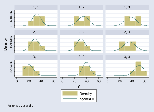
histogram y, by(a b) normal
 anova y a b a#b
Number of obs = 45 R-squared = 0.5690
Root MSE = 7.90569 Adj R-squared = 0.4732
Source | Partial SS df MS F Prob > F
-----------+----------------------------------------------------
Model | 2970 8 371.25 5.94 0.0001
|
a | 190 2 95 1.52 0.2324
b | 1543.33333 2 771.666667 12.35 0.0001
a#b | 1236.66667 4 309.166667 4.95 0.0028
|
Residual | 2250 36 62.5
-----------+----------------------------------------------------
Total | 5220 44 118.636364
effectsize b
anova effect size for b with dep var = y
total variance accounted for
omega2 = .26849661
eta2 = .29565773
Cohen's f = .60584458
partial variance accounted for
partial omega2 = .33523734
partial eta2 = .40685413
effectsize a#b
anova effect size for a#b with dep var = y
total variance accounted for
omega2 = .18678025
eta2 = .23690932
Cohen's f = .47924933
partial variance accounted for
partial omega2 = .25970608
partial eta2 = .35468451
anova y a b a#b
Number of obs = 45 R-squared = 0.5690
Root MSE = 7.90569 Adj R-squared = 0.4732
Source | Partial SS df MS F Prob > F
-----------+----------------------------------------------------
Model | 2970 8 371.25 5.94 0.0001
|
a | 190 2 95 1.52 0.2324
b | 1543.33333 2 771.666667 12.35 0.0001
a#b | 1236.66667 4 309.166667 4.95 0.0028
|
Residual | 2250 36 62.5
-----------+----------------------------------------------------
Total | 5220 44 118.636364
effectsize b
anova effect size for b with dep var = y
total variance accounted for
omega2 = .26849661
eta2 = .29565773
Cohen's f = .60584458
partial variance accounted for
partial omega2 = .33523734
partial eta2 = .40685413
effectsize a#b
anova effect size for a#b with dep var = y
total variance accounted for
omega2 = .18678025
eta2 = .23690932
Cohen's f = .47924933
partial variance accounted for
partial omega2 = .25970608
partial eta2 = .35468451Plotting Cell Means
anovaplot b a, scatter(msym(none)) /* findit anovaplot */Stata Regression Resultsanovaplot a b, scatter(msym(none)) /* findit anovaplot */
regress y x1 x2 x3 x4 x5 x6 x7 x8

  Source |       SS       df       MS                  Number of obs =      45
---------+------------------------------               F(  8,    36) =    5.94
   Model |     2970.00     8      371.25               Prob > F      =  0.0001
Residual |     2250.00    36       62.50               R-squared     =  0.5690
---------+------------------------------               Adj R-squared =  0.4732
   Total |     5220.00    44  118.636364               Root MSE      =  7.9057

------------------------------------------------------------------------------
       y |      Coef.   Std. Err.       t     P>|t|       [95% Conf. Interval]
---------+--------------------------------------------------------------------
      x1 |        1.5   1.443376      1.039   0.306      -1.427302    4.427302
      x2 |  -1.166667   .8333333     -1.400   0.170      -2.856745    .5234117
      x3 |  -3.833333   1.443376     -2.656   0.012      -6.760635   -.9060318
      x4 |       -3.5   .8333333     -4.200   0.000      -5.190078   -1.809922
      x5 |       -.25   1.767767     -0.141   0.888      -3.835198    3.335198
      x6 |        .25   1.020621      0.245   0.808      -1.819915    2.319915
      x7 |   3.083333   1.020621      3.021   0.005       1.013419    5.153248
      x8 |   1.916667   .5892557      3.253   0.002       .7216008    3.111733
   _cons |         35   1.178511     29.698   0.000       32.60987    37.39013
------------------------------------------------------------------------------

test x1 x2

 ( 1)  x1 = 0.0
 ( 2)  x2 = 0.0

       F(  2,    36) =    1.52
            Prob > F =    0.2324

test x3 x4

 ( 1)  x3 = 0.0
 ( 2)  x4 = 0.0

       F(  2,    36) =   12.35
            Prob > F =    0.0001

test x5 x6 x7 x8

 ( 1)  x5 = 0.0
 ( 2)  x6 = 0.0
 ( 3)  x7 = 0.0
 ( 4)  x8 = 0.0

       F(  4,    36) =    4.95
            Prob > F =    0.0028

xi3: regress y r.a*r.b
r.a               _Ia_1-3             (naturally coded; _Ia_1 omitted)
r.b               _Ib_1-3             (naturally coded; _Ib_1 omitted)
r.a*r.b           _IaXb_#_#           (coded as above)

      Source |       SS       df       MS              Number of obs =      45
-------------+------------------------------           F(  8,    36) =    5.94
       Model |     2970.00     8      371.25           Prob > F      =  0.0001
    Residual |     2250.00    36       62.50           R-squared     =  0.5690
-------------+------------------------------           Adj R-squared =  0.4732
       Total |     5220.00    44  118.636364           Root MSE      =  7.9057

------------------------------------------------------------------------------
           y |      Coef.   Std. Err.      t    P>|t|     [95% Conf. Interval]
-------------+----------------------------------------------------------------
       _Ia_2 |         -3   2.886751    -1.04   0.306    -8.854603    2.854603
       _Ia_3 |        3.5        2.5     1.40   0.170    -1.570235    8.570235
       _Ib_2 |   7.666667   2.886751     2.66   0.012     1.812064    13.52127
       _Ib_3 |       10.5        2.5     4.20   0.000     5.429765    15.57023
   _IaXb_2_2 |         -1   7.071068    -0.14   0.888    -15.34079    13.34079
   _IaXb_2_3 |        1.5   6.123724     0.24   0.808    -10.91949    13.91949
   _IaXb_3_2 |       18.5   6.123724     3.02   0.005     6.080511    30.91949
   _IaXb_3_3 |      17.25   5.303301     3.25   0.002     6.494407    28.00559
       _cons |         35   1.178511    29.70   0.000     32.60987    37.39013
------------------------------------------------------------------------------

describe _Ia_2 - _IaXb_3_3

              storage  display     value
variable name   type   format      label      variable label
-------------------------------------------------------------------------------
_Ia_2           double %10.0g                 a(2 vs. 1)
_Ia_3           double %10.0g                 a(3 vs. 2-)
_Ib_2           double %10.0g                 b(2 vs. 1)
_Ib_3           double %10.0g                 b(3 vs. 2-)
_IaXb_2_2       double %10.0g                 a(2 vs. 1) & b(2 vs. 1)
_IaXb_2_3       double %10.0g                 a(2 vs. 1) & b(3 vs. 2-)
_IaXb_3_2       double %10.0g                 a(3 vs. 2-) & b(2 vs. 1)
_IaXb_3_3       double %10.0g                 a(3 vs. 2-) & b(3 vs. 2-)

test _Ia_2 _Ia_3

 ( 1)  _Ia_2 = 0.0
 ( 2)  _Ia_3 = 0.0

       F(  2,    36) =    1.52
            Prob > F =    0.2324

test _Ib_2 _Ib_3

 ( 1)  _Ib_2 = 0.0
 ( 2)  _Ib_3 = 0.0

       F(  2,    36) =   12.35
            Prob > F =    0.0001

test _IaXb_2_2 _IaXb_2_3 _IaXb_3_2 _IaXb_3_3

 ( 1)  _IaXb_2_2 = 0.0
 ( 2)  _IaXb_2_3 = 0.0
 ( 3)  _IaXb_3_2 = 0.0
 ( 4)  _IaXb_3_3 = 0.0

       F(  4,    36) =    4.95
            Prob > F =    0.0028
Stata Regression with anovalator
regress y i.a##i.b


      Source |       SS       df       MS              Number of obs =      45
-------------+------------------------------           F(  8,    36) =    5.94
       Model |        2970     8      371.25           Prob > F      =  0.0001
    Residual |        2250    36        62.5           R-squared     =  0.5690
-------------+------------------------------           Adj R-squared =  0.4732
       Total |        5220    44  118.636364           Root MSE      =  7.9057

------------------------------------------------------------------------------
           y |      Coef.   Std. Err.      t    P>|t|     [95% Conf. Interval]
-------------+----------------------------------------------------------------
           a |
          2  |         -3          5    -0.60   0.552    -13.14047     7.14047
          3  |        -13          5    -2.60   0.013    -23.14047    -2.85953
             |
           b |
          2  |          2          5     0.40   0.692     -8.14047    12.14047
          3  |          5          5     1.00   0.324     -5.14047    15.14047
             |
         a#b |
        2 2  |         -1   7.071068    -0.14   0.888    -15.34079    13.34079
        2 3  |          1   7.071068     0.14   0.888    -13.34079    15.34079
        3 2  |         18   7.071068     2.55   0.015      3.65921    32.34079
        3 3  |         27   7.071068     3.82   0.001     12.65921    41.34079
             |
       _cons |         33   3.535534     9.33   0.000      25.8296     40.1704
------------------------------------------------------------------------------

anovalator a b, main 2way fratio

anovalator main-effect for a
chi2(2) = 3.04   p-value = .21871189
scaled as F-ratio = 1.52

anovalator main-effect for b
chi2(2) = 24.693333   p-value = 4.344e-06
scaled as F-ratio = 12.346667

anovalator two-way interaction for a#b
chi2(4) = 19.786667   p-value = .00055023
scaled as F-ratio = 4.9466667
FormulasLinear model,

Prediction model,
where,
thus,
Linear Statistical Models Course
Phil Ender, 11apr06, 12Feb98