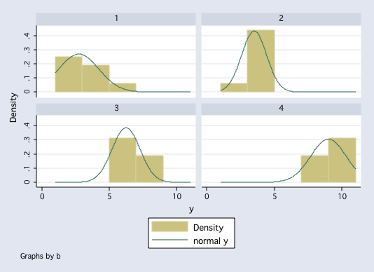
histogram y, by(b) normal
pnorm y if b==1
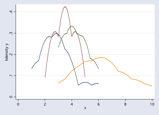
twoway (kdensity y if b==1)(kdensity y if b==2)(kdensity y if b==3)(kdensity y if b==4), legend(off))
Three Universal Assumptions of Analysis of Variance
Independence
Independence is verified by checking on how subjects were selected and how they were assigned to groups. If subjects are randomly sampled and randomly assigned to groups then the independence assumption is easily met. If some other method is used to sample and assign subjects then it is necessary to examine the procedure closely to determine whether the assumption of independence is still met.
Normality
Althought tests exist for checking normality, it is probably as effective to visually inspect distribution graphs for each group.
twoway (kdensity y if b==1)(kdensity y if b==2)(kdensity y if b==3)(kdensity y if b==4), legend(off))
The tricky part is when group sample sizes are small. In these cases it is difficult to tell whether the sample was drawn from a normally distributed population or not.
Example Histograms of Random Samples
Homogeneity of Variance
This assumption is also called homoscedasicity. For this assumption, we need to check to see if the population variances for each of the groups from which the samples were drawn have equal variances.
Althought a number of tests exist for checking homogeneity of variance, most if not all of them are affected to some degree by non-normality in the samples. It is not recommended that tests of homogeneity of variance be run as a matter of course. It is usually safer to inspect the variances or standard deviations for each group. If the ratio of the variances differ by more than nine or the ratio of the standard deviations differ by more than three, then the researcher should be concerned about heterogeneity of variance.
Here are four methods for checking the homogeneity of variance assumption. Of the four, Levene's test is least affected by non-normality.
Table of Group Means, Variances and Standard Deviations
tabstat y, by(a) stat(n mean sd var)

       b |         N      mean        sd  variance
---------+----------------------------------------
       1 |         8      2.75  1.488048  2.214286
       2 |         8       3.5  .9258201  .8571429
       3 |         8      6.25  1.035098  1.071429
       4 |         8         9  1.309307  1.714286
---------+----------------------------------------
   Total |        32     5.375  2.756225  7.596774
--------------------------------------------------
Fmax Test for Homogeneity of Variance
with df = p & (n-1) Table of Fmax
From the Example:
Fmax = 2.214/0.857 = 2.58
with 4 & 7 degrees of freedom.
Bartlett's Test for Homogeneity of Variance
From the Example:
B = 1.8281 (as computed by STATA)
with k - 1 = 3 degrees of freedom.
Cochran's Test for Homogeneity of Variance
df = k and n - 1 (the same as Fmax)
From the Example:
C = 2.214/5.856 = .3781
with 4 & 7 degrees of freedom.
Levene's's Test for Homogeneity of Variance
Perform one-way ANOVA using d as the dependent variable.
From the Example:
F = 1.29, p = 0.2963
with 3 & 28 degrees of freedom.
robvar y, by(a)

            |            Summary of y
          a |        Mean   Std. Dev.       Freq.
------------+------------------------------------
          1 |           3   1.5118579           8
          2 |         3.5    .9258201           8
          3 |        4.25   1.0350983           8
          4 |        6.25   2.1213203           8
------------+------------------------------------
      Total |        4.25   1.8837163          32

W0  = 1.292876   df(3, 28)     Pr > F = .29625408  /*  <-- this is the Levene's test */

W50 = 1.037037   df(3, 28)     Pr > F = .39138742

W10 = 1.292876   df(3, 28)     Pr > F = .29625408
Levene's F is a relatively robust measure of
homogeneity of variance. It was not really needed in
this example because the standard deviations are so
close together. The other tests of homoscedasticity, F-max, Bartlett's test, and Cochrans's,
are more strongly influenced by
non-normality than is Levene's test.
The first step in checking on the assumption of
homogeneity of variance should be to inspect
the standard deviations or variances within each level.Exploring Robustness
A statistical test is said to be robust if it yields correct conclusions even when some of the assumptions are not met. Generally, anova is considered to be relatively robust to violations of normality and homogeneity, especially when the sample sizes are equal or nearly equal.
We can explore the robustness of some one-way designs to heterscedasiticty and sample size using simanova. simanova performs a Monte Carlo simulation of completely randomized designs under the assumption that the group means are equal. We can compare the observed proportion of tests that fall into each of sevear nominal alpha levels.
net from http://www.ats.ucla.edu/stat/stata/ado/analysis
net install simanova

use http://www.philender.com/courses/data/cr4new, clear

anova y a

                           Number of obs =      32     R-squared     =  0.4455
                           Root MSE      =   1.476     Adj R-squared =  0.3860

                  Source |  Partial SS    df       MS           F     Prob > F
              -----------+----------------------------------------------------
                   Model |          49     3  16.3333333       7.50     0.0008
                         |
                       a |          49     3  16.3333333       7.50     0.0008
                         |
                Residual |          61    28  2.17857143
              -----------+----------------------------------------------------
                   Total |         110    31   3.5483871

simanova y a

Information about Sample Sizes and Standard Deviations
------------------------------------------------------
N1 = 8 and S1 = 1.5118579
N2 = 8 and S2 = .92582011
N3 = 8 and S3 = 1.0350983
N4 = 8 and S4 = 2.1213202

Results of Standard ANOVA

----------------------------------------------------------------------
Dependent Variable is y and Independent Variable is a
F(  3,  28.00) =   7.497, p= 0.0008
----------------------------------------------------------------------

         1000 simulated ANOVA F tests
         --------------------------------
Nominal  Simulated   Simulated P value
P Value  P Value     [95% Conf. Interval]
-----------------------------------------
 0.0008   0.0010       0.0000 - 0.0056
 0.2000   0.2160       0.1909 - 0.2428
 0.1000   0.1200       0.1005 - 0.1418
 0.0500   0.0600       0.0461 - 0.0766
 0.0100   0.0110       0.0055 - 0.0196

simanova, gr(4) n(8 8 8 8) s(1 1 1 3)

Information about Sample Sizes and Standard Deviations
------------------------------------------------------
N1 = 8 and S1 = 1
N2 = 8 and S2 = 1
N3 = 8 and S3 = 1
N4 = 8 and S4 = 3

         1000 simulated ANOVA F tests
         --------------------------------
Nominal  Simulated   Simulated P value
P Value  P Value     [95% Conf. Interval]
-----------------------------------------
 0.2000   0.2110       0.1861 - 0.2376
 0.1000   0.1300       0.1098 - 0.1524
 0.0500   0.0790       0.0630 - 0.0975
 0.0100   0.0440       0.0321 - 0.0586

simanova, gr(4) n(8 8 8 8) s(1 1 1 9)

Information about Sample Sizes and Standard Deviations
------------------------------------------------------
N1 = 8 and S1 = 1
N2 = 8 and S2 = 1
N3 = 8 and S3 = 1
N4 = 8 and S4 = 9

         1000 simulated ANOVA F tests
         --------------------------------
Nominal  Simulated   Simulated P value
P Value  P Value     [95% Conf. Interval]
-----------------------------------------
 0.2000   0.2340       0.2081 - 0.2615
 0.1000   0.1610       0.1387 - 0.1853
 0.0500   0.1190       0.0996 - 0.1407
 0.0100   0.0570       0.0435 - 0.0732

simanova, gr(4) n(16 16 16 8) s(1 1 1 9)

Information about Sample Sizes and Standard Deviations
------------------------------------------------------
N1 = 16 and S1 = 1
N2 = 16 and S2 = 1
N3 = 16 and S3 = 1
N4 = 8 and S4 = 9

         1000 simulated ANOVA F tests
         --------------------------------
Nominal  Simulated   Simulated P value
P Value  P Value     [95% Conf. Interval]
-----------------------------------------
 0.2000   0.3950       0.3646 - 0.4261
 0.1000   0.3370       0.3077 - 0.3672
 0.0500   0.2850       0.2572 - 0.3141
 0.0100   0.1930       0.1690 - 0.2188
Linear Statistical Models Course
Phil Ender, 4apr06, 4jun99; 15mar02