Introduction to Research Design and Statistics
Probability
Random Phenomenon / Random Process
When individual outcomes are uncertain but there are nonetheless regular
distributions of relative frequencies over a large number of trials.
Probability
In intuitive terms, long-term relative frequency
Probability Distribution
A set of probabilities associated with all possible outcomes of a variable.
Probability distributions are abstract mathematical models which are useful
to the extent to which they reflect distributions of variables in the real world.
Probability Models
Sample Space
- The set of all possible outcomes of a random phenomenon.
- Denoted S.
Random Variable
A random variable is a numerial outcome of a random process whose exact
value cannot be predicted exactly beforehand.
Event
- A set of outcomes of a random process.
i.e., a subset of the sample space.
Example:
Tossing three coins.
[{TTT} {TTH} {THT} {HTT} {THH} {HTH} {HHT} {HHH}]
Each of the above is an event.
All of the above, taken together, constitute the sample space.
Probability Rule #1
0<=P(A)<=1
Probability Rule #2
P(S) = 1
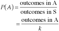
Equally Likely Outcomes
If a random phenomenon has k possible outcomes, all equally likely,
than each individual outcome has the probability of 1/k. The
probability of any event A is

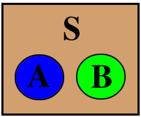
Disjoint Events
(Mutually Exclusive Events)
Events that have no outcomes in common.
Venn Diagram
A picture used to make probability incomprehensible.

A and B are disjoint
Probability Rule #3
Addition Rule for Disjoint Events
If event A and B are disjoint,
then P(A or B) = P(A) + P(B)
Example:
In tossing 3 coins what is the probability that there will be all heads or no heads?
[{TTT} {TTH} {THT} {HTT} {THH} {HTH} {HHT} {HHH}]
P(A)=1/8 P(B)=1/8
P(A) + P(B) = 2/8 = 1/4
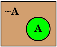
Complement of an Event
- What a simply marvelous party this is.
- For any event A, the event that A does not happen.
- Denoted AC or ~A
Another Venn Diagram

Probability Rule #4
The Complement Rule
For any event A, the probability of ~A is
Example:
In tossing 3 coins, what is the probability that there will not be exactly one head.
Event A is exactly one head.
[{TTT} {TTH} {THT} {HTT} {THH} {HTH} {HHT} {HHH}]
P(A) = 3/8
P(~A) = 1 - 3/8 = 5/8
Independent Events
Events A and B are independent if knowledge about the outcome of A
does not change the probability of B.
Example:
- Tossing a coin twice.
- Picking 2 cards from a deck.
- Which are independent?
Probability Rule #5
Multiplication Rule for Independent Events
If A and B are independent,
then P(A and B) = P(A)P(B)
Example:
Pick a card at random from a deck of cards.
What is the probability that the card will be black and an ace.
Event A is card is black; Event B is card is an Ace
P(A) = 26/52 P(B) = 4/52
P(A and B) = 104/2704 = 2/52
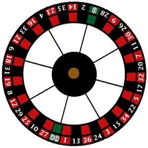
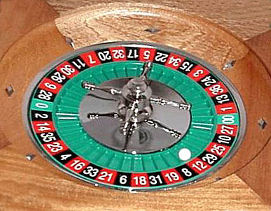
How Las Vegas Makes Money


Random Variables
Random Variable
A variable whose value is a numerical outcome of a random phenomenon.
Discrete Random Variables
- A discrete random variable X takes a finite number of values, x1, x2, ..., xk
- The probability pi is assigned to each event xi
- The sum of all the pi is 1.0
Probability Distribution
The set of probabilities assigned to a random variable X.
Example:
Number of Heads in Tossing 3 Coins
#Heads          Prob
  xi             pi
  0             1/8
  1             3/8
  2             3/8
  3             1/8
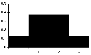
Probability Histogram
A graphical representation of the probability distribution of a discrete random variable.
Example:
Number of Heads in Tossing 3 Coins

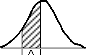
Continuous Random Variable
- A continuous random variable X takes all values in an interval of real numbers
- The probability P(A) is equal to the area above the interval A and under the curve
- The total area under the curve is 1.0
Example:

Normal Distributions
- A normal probability distribution is one of the most common examples of a
continuous random variable.
- Probabilities associated with different intervals are found in tables of normal
probabilities.
Means & Variances of Random Variables
Expected Value
- The mean of a random variable
- Denoted E(X)
Mean
Discrete Random Variable
mx = E(X) = Σxipi
Example:
Number of heads in tossing three coins.
#Heads     Prob     Product
    xi      pi
    0      1/8         0
    1      3/8        3/8
    2      3/8        6/8
    3      1/8        3/8
               Sum = 12/8 = 1.5 = E(X) = μx
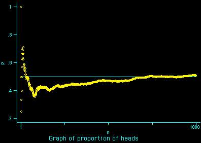
Law of Large Numbers
The observed mean outcome in many independent
trials must approach the mean of the probability distribution.

Rule #1 for Means
When Y = a + bX
Rule #2 for Means
When Z = X + Y
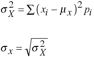
Variance
Discrete Random Variable

Example:
Number of Heads in Tossing 3 Coins
#Heads     (xi-μ)2      Prob     Product
   0         2.25       1/8        0.28
   1         0.25       3/8        0.09
   2         0.25       3/8        0.09
   3         2.25       1/8        0.28
                  Sum = Variance = 0.74
              Standard Deviation = 0.87
Rule #1 for Variances
When Y = a + bX
Rule #2 for Variances
When Z = X + Y and X & Y are independent
Rule #2a for Variances
When Z = X - Y and X & Y are independent
Intro Home Page
Phil Ender, 18Nov99
