With appologies to Fredrick Lord* here is my take on football numbers.

*Lord, F. (1953) On the statistical treatment of football numbers. American Psychologist, 8, 750-751.

I have entered the following data from the 2002 UCLA football team roster: jersey number, last name, height (in inches), weight (in pounds), position.

Weight and height are both ratio scaled variables while jersey number is nominally scaled. That is, the numbers on the football jerseys are used for identification, they do not indicate an amount or quantity of something. Or do they?

Let's analyze these data.

use http://www.philender.com/courses/data/football, clear
 
summarize wt ht jnum

    Variable |     Obs        Mean   Std. Dev.       Min        Max
-------------+-----------------------------------------------------
          wt |      92    231.1957   42.48859        155        330
          ht |      92    74.20652   2.703429         67         81
        jnum |      92    44.45652   29.37795          1         99
 
tabstat wt ht jnum, stat(mean p25 median p75) col(stat)

    variable |      mean       p25       p50       p75
-------------+----------------------------------------
          wt |  231.1957     196.5       226     269.5
          ht |  74.20652      72.5        74        76
        jnum |  44.45652        19      41.5      71.5
------------------------------------------------------
 
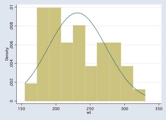
histogram wt, bin(10) normal
 

 
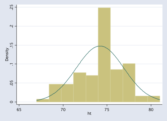
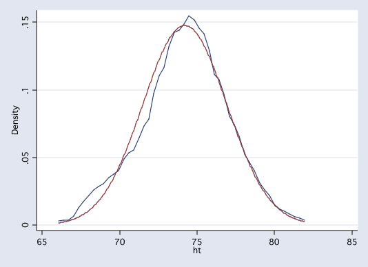
histogram ht, bin(10) normal
 

 
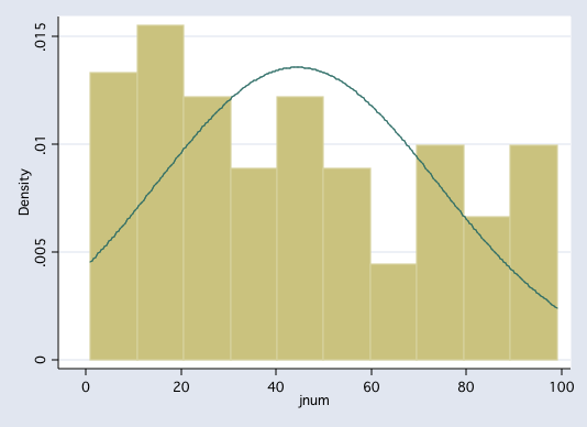
histogram jnum, bin(10) normal
 

 
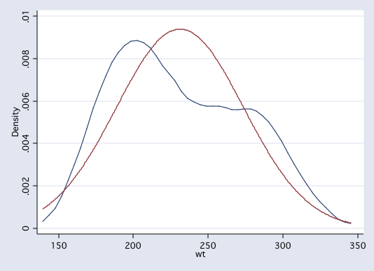
kdensity wt, normal legend(off)
 

 
kdensity ht, normal legend(off)
 

 
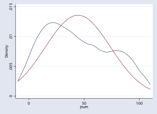
kdensity jnum, normal legend(off)
 

 
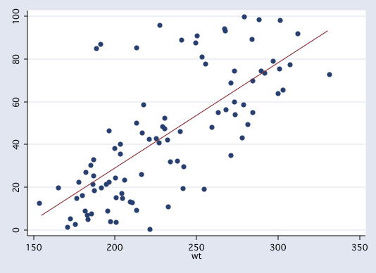
twoway (scatter jnum wt, jitter(2))(lfit jnum wt), legend(off)
 

 
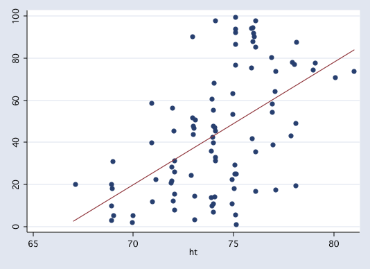
twoway (scatter jnum ht, jitter(2))(lfit jnum ht), legend(off)
 

 
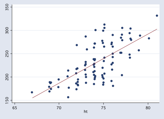
twoway (scatter wt ht, jitter(2))(lfit wt ht), legend(off)
 

 
corr jnum wt ht
(obs=92)

             |     jnum       wt       ht
-------------+---------------------------
        jnum |   1.0000
          wt |   0.7119   1.0000
          ht |   0.5330   0.6716   1.0000

Now, as a comparison, let's create a data set that has each of the numbers from 1 to 99, remember no two players can have the same number.

clear
set obs 99
gen x=_n
summarize x
 
    Variable |     Obs        Mean   Std. Dev.       Min        Max
-------------+-----------------------------------------------------
           x |      99          50   28.72281          1         99
 
tabstat x, stat(mean p25 median p75)
 
    variable |      mean       p25       p50       p75
-------------+----------------------------------------
           x |        50        25        50        75
------------------------------------------------------

In a uniform or rectangular distribution the mean is (max+min)/2 = (1+99)/2 = 50 and the variance is (max-min)^2/12 = (99-1)^2/12 = 800.33333. The standard deviation is the square root of the variance = sqrt(800.33333) = 28.290163. This value is slightly different from the 28.72281 above. The value computed by Stata is the unbiased estimate of the population standard deviation while the 28.290163 is the population standard deviation.

Intro Home Page