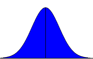

The normal probability distribution is a mathematical model which is generated by a specific mathematical function. This mathematical model is useful because many variables observed in nature closely approximate a normal distribution.
Normal distributions are symmetric and the tails are asymptotic, that is, the tails approach the baseline but never quite reach it no matter how far away from the mean you are. Obviously, our illustrations do not completely capture the nature of normal distributions.

The standard normal distribution has a mean of zero (mean = 0) and a variance of one (s2 = 1) thus, of course, the standard deviation is one (s = 1).
Since most distributions are observed rather than generated mathematically, there are features of normal distributions that can also be observed. In a normal distribution 68.26% of the distribution will fall between plus and minus one standard deviation (±1.0s). Usually, this will be denoted using the standard normal (Z-score) distribution as ±1.0Z. Here are some other values form the standard normal distribution, 95.44% between ±2.0Z and 99.74% between ±3.0Z.
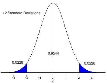
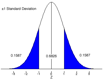
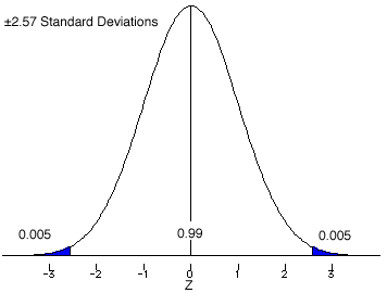

The easy way to find the areas (probabilities) under the standard normal curve are to use the tables found in every statistics book. These tables can be formatted several different ways. We will use a method that displays the area between the mean (Z = 0.0) and a given Z-score.
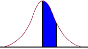
The command ztable displays the areas under the standard normal curve from the mean to the value of z. ztable can be downloaded from ATS via the Internet using these commands:
net from http://www.ats.ucla.edu/stat/stata/ado/teach/
net install probtabl
Here is part of the display from the ztable command:
ztable

      Areas between 0 & Z of the Standard Normal Distribution
      .00    .01    .02    .03    .04   |  .05    .06    .07    .08    .09
0.00 0.0000 0.0040 0.0080 0.0120 0.0160 | 0.0199 0.0239 0.0279 0.0319 0.0359
0.10 0.0398 0.0438 0.0478 0.0517 0.0557 | 0.0596 0.0636 0.0675 0.0714 0.0753
0.20 0.0793 0.0832 0.0871 0.0910 0.0948 | 0.0987 0.1026 0.1064 0.1103 0.1141
0.30 0.1179 0.1217 0.1255 0.1293 0.1331 | 0.1368 0.1406 0.1443 0.1480 0.1517
0.40 0.1554 0.1591 0.1628 0.1664 0.1700 | 0.1736 0.1772 0.1808 0.1844 0.1879
0.50 0.1915 0.1950 0.1985 0.2019 0.2054 | 0.2088 0.2123 0.2157 0.2190 0.2224
0.60 0.2257 0.2291 0.2324 0.2357 0.2389 | 0.2422 0.2454 0.2486 0.2517 0.2549
0.70 0.2580 0.2611 0.2642 0.2673 0.2704 | 0.2734 0.2764 0.2794 0.2823 0.2852
0.80 0.2881 0.2910 0.2939 0.2967 0.2995 | 0.3023 0.3051 0.3078 0.3106 0.3133
0.90 0.3159 0.3186 0.3212 0.3238 0.3264 | 0.3289 0.3315 0.3340 0.3365 0.3389
1.00 0.3413 0.3438 0.3461 0.3485 0.3508 | 0.3531 0.3554 0.3577 0.3599 0.3621
Note: Graphs are designed to give a rough estimate and are not drawn to exact scale or proportion.
1. In this sample, how many students would be expected to score above Paul?
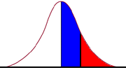
2. What proportion of the students would be expected to score above John?
3. What percent of students would be expected to score above Ringo?
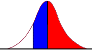
4. How many students would be expected to score below Ringo?
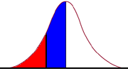
5. What percentage of students would be expected to score below George?
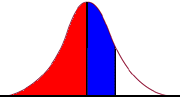
6. What proportion of students would be expected to score below John?
7. How many students would be expected to score between George and Ringo?

8. What proportion of students would be expected to score between John and Paul?
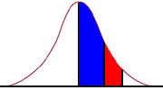
9. What percentage of students would be expected to score between George and Paul?
10. 225 students score above Linda, what is her test score?
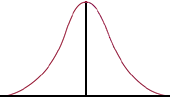
11. What are the approximate test scores for Q1 and Q3?
12. A middle-school student took two standardized tests. On the Language Proficiency test she scored 114.4 (mean = 100, sd = 16) and on Mathematical Reasoning she scored 61.7 (mean = 50, sd = 9). On which test did she do better?
Intro Home Page
Phil Ender, 30Jun98