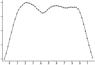
Figure 1: Population Distribution
  Variable |     Obs        Mean   Std. Dev.       Min        Max
-----------+-------------------------------------------------------
Population |    1000    .5000000   .2886751   .0000000   1 .0000000
    n =  5 |    1000    .5036115   .125487    .106075      .8491938
    n = 20 |    1000    .5000545   .0637908   .2998779     .6954108
    n = 36 |    1000    .5044926   .048932    .3551762     .6496101
Here are plots of the population and each of the sampling distributions:

Figure 1: Population Distribution
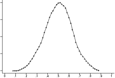
Figure 2: Sampling Distribution for n = 5
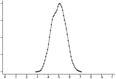
Figure 3: Sampling Distribution for n = 20
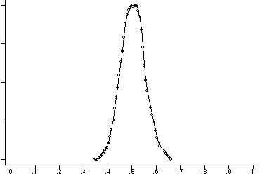
Figure 4: Sampling Distribution for n = 36
Now let's try repeat the process of drawing 1,000 samples of n = 5, n = 20 and n = 36 from a highly skewed population:
  Variable |     Obs        Mean   Std. Dev.       Min        Max
-----------+-------------------------------------------------------
Population |    1000    1.088532   .6348374   .1219511   4.914284
    n =  5 |    1000    1.11774    .3052395   .3961306   2.660268
    n = 20 |    1000    1.116671   .1449324   .7067162   1.773374
    n = 36 |    1000    1.108628   .1043764   .8531538   1.515452
Here are plots of the population and each of the sampling distributions:
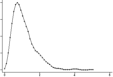
Figure 5: Population Distribution
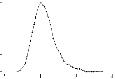
Figure 6: Sampling Distribution for n = 5
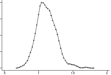
Figure 7: Sampling Distribution for n = 20
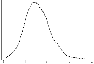
Figure 8: Sampling Distribution for n = 36
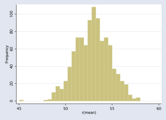
use http://www.philender.com/courses/data/lahigh, clear histogram daysatt, freq discretebs "summarize daysatt" "r(mean)",reps(1000) size(150) saving(mybs) command: summarize daysatt statistic: r(mean) (obs=316) Bootstrap statistics Variable | Reps Observed Bias Std. Err. [95% Conf. Interval] ---------+------------------------------------------------------------------- bs1 | 1000 74.65823 -.0141592 .9349639 72.82351 76.49294 (N) | 72.78667 76.37667 (P) | 72.72 76.34666 (BC) ----------------------------------------------------------------------------- N = normal, P = percentile, BC = bias-corrected use mybs histogram bs1, freq
Intro Home Page
Phil Ender, 30Jun98