Interval Estimation

Introduction to Research Design and Statistics

Interval Estimation

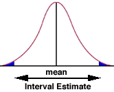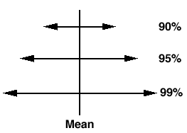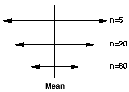
Estimating the population mean by using the sample mean is called point estimation. It is also possible to do another type of estimation, interval estimation. In interval estimation, also called confidence intervals, one gives a range of values along with a level of confidence.

Confidence Interval

A confidence interval for a parameter is an interval computed from sample data containing the true value of the parameter with a certain level of confidence.

With a 95% confidence interval for a sample mean, 95% of all sample of the same size will contain the true population mean. Which is very close to saying that the true population mean has a 95% chance of falling within the confidence interval (close but not exactly the same).

A confidence interval has the form:

estimate ± margin of error

Level of Confidence

The researcher selects a level of confidence to be used in interval estimation. In general, the greater the degree of confidence the wider the confidence interval must be. Typical confidence levels are 90% (.90), 95% (.95), and 99% (.99). Confidence levels are related to the alpha level, alpha = 1 - confidence level. Example alpha = 1 - .95 = .05.

Constructing a Single Sample Confidence Interval for the Mean

Or more simply:

use df = n-1

About Confidence Intervals

Confidence intervals get wider as the confidence increases:

Confidence intervals get narrower as sample size increases:

Example

A sample of 64 students were able to finish a geometry test in an average time of 27.75 minutes with a standard deviation of 5.083.

Construct a 95% confidence interval using the sample mean.

Next, compute the standard error of the mean:
se = s/SQRT(n) =5.083/SQRT(64) = 0.635

Construct the confidence interval:
Xbar ± CVt * se = 27.75 ± 2.00*0.635 = 27.75 ± 1.27
(26.48, 29.03)

Example Using Stata

cii 64 27.75 5.083

Variable |     Obs         Mean    Std. Err.       [95% Conf. Interval]
---------+-------------------------------------------------------------
         |      64        27.75     .635375         26.4803     29.0197

Confidence Intervals and Hypothesis Testing

A 95% confidence interval is equivalent to a two-tail test of hypotheses at alpha = 0.05. If the hypothesized population mean falls outside of the confidence then the null hypothesis is rejected.

Test the hypothesis that the sample comes from a population with a mean of 33.02.

The hypothesized popluation mean is 33.02 which falls outside of the 95% confidence interval.

Therefore, reject the null hypothesis at alpha = 0.05.

Cautions

Data should be taken from a simple random sample.

Only takes into account sampling variability, not bias.

Is not resistant to outliers.

Small samples are influenced by skewness.

Confidence Interval for the Difference in Means

Use df = n₁ + n₂ - 2

Remember:

Pooled Variance:

Standard Error of the Differences Between Means

Example

Experimental Group: Phonics, n = 15, mean = 50, s = 8.7
Control Group: Whole Language, n = 17, mean 45, s = 5.9

Construct a 95% confidence interval on the difference in means.

₁

₂

Next, compute the standard error of the differences in means:
s_p² = ((15-1)*8.7²+(17-1)*5.9²)/(15+17-2)= (1,059.66+556.96)/30 = 1,616.62/30 = 53.89
s_p = SQRT(s_p²) = SQRT(53.89) = 7.34

se = s_p*SQRT(1/n₁ + 1/n₂) = 7.34*SQRT(1/15 + 1/17) = 2.6

Construct the confidence interval:
Xbar₁ - Xbar₂ ± CVt * se = 50 - 45 ± 2.042*2.6 = 5 ± 5.31
(-0.31, 10.31)

Example Using Stata

ttesti 15 50 8.7 17 45 5.9

Two-sample t test with equal variances

------------------------------------------------------------------------------
         |     Obs        Mean    Std. Err.   Std. Dev.   [95% Conf. Interval]
---------+--------------------------------------------------------------------
       x |      15          50     2.24633         8.7     45.1821     54.8179
       y |      17          45     1.43096         5.9     41.9665     48.0335
---------+--------------------------------------------------------------------
combined |      32    47.34375    1.352953     7.65346    44.58438    50.10312
---------+--------------------------------------------------------------------
    diff |                   5    2.600448               -.3108242    10.31082
------------------------------------------------------------------------------
Degrees of freedom: 30

                      Ho: mean(x) - mean(y) = diff = 0

     Ha: diff < 0               Ha: diff ~= 0              Ha: diff > 0
       t =   1.9227                t =   1.9227              t =   1.9227
   P < t =   0.9680          P > |t| =   0.0641          P > t =   0.0320

Confidence Intervals and Hypothesis Testing Again

A 95% confidence interval is equivalent to a two-tail test of hypotheses at alpha = 0.05. If zero, the hypothesized difference in population means, falls outside of the confidence then the null hypothesis is rejected.

Test the hypothesis that the two samples come from a populations with equal means.

The hypothesized difference in popluation means, zero, does not fall outside the 95% confidence interval.

Therefore, fail to reject reject the null hypothesis at alpha = 0.05.

More Stata Examples

use http://www.philender.com/courses/data/hsb2, clear
 

ci read write math science socst

Variable |     Obs         Mean    Std. Err.       [95% Conf. Interval]
---------+-------------------------------------------------------------
    read |     200        52.23    .7249921        50.80035    53.65965
   write |     200       52.775    .6702372        51.45332    54.09668
    math |     200       52.645    .6624493        51.33868    53.95132
 science |     200        51.85    .7000987        50.46944    53.23056
   socst |     200       52.405    .7591352        50.90802    53.90198
 
ci read write math science socst, level(90)

Variable |     Obs         Mean    Std. Err.       [90% Conf. Interval]
---------+-------------------------------------------------------------
    read |     200        52.23    .7249921        51.03192    53.42808
   write |     200       52.775    .6702372         51.6674     53.8826
    math |     200       52.645    .6624493        51.55027    53.73973
 science |     200        51.85    .7000987        50.69305    53.00695
   socst |     200       52.405    .7591352        51.15049    53.65951
 
ci read write math science socst, level(99)

Variable |     Obs         Mean    Std. Err.       [99% Conf. Interval]
---------+-------------------------------------------------------------
    read |     200        52.23    .7249921        50.34447    54.11553
   write |     200       52.775    .6702372        51.03187    54.51813
    math |     200       52.645    .6624493        50.92213    54.36787
 science |     200        51.85    .7000987        50.02921    53.67079
   socst |     200       52.405    .7591352        50.43067    54.37933
 
ttest write, by(female)

Two-sample t test with equal variances

------------------------------------------------------------------------------
   Group |     Obs        Mean    Std. Err.   Std. Dev.   [95% Conf. Interval]
---------+--------------------------------------------------------------------
    male |      91    50.12088    1.080274    10.30516    47.97473    52.26703
  female |     109    54.99083    .7790686    8.133715    53.44658    56.53507
---------+--------------------------------------------------------------------
combined |     200      52.775    .6702372    9.478586    51.45332    54.09668
---------+--------------------------------------------------------------------
    diff |           -4.869947    1.304191               -7.441835   -2.298059
------------------------------------------------------------------------------
Degrees of freedom: 198

                  Ho: mean(male) - mean(female) = diff = 0

     Ha: diff < 0               Ha: diff ~= 0              Ha: diff > 0
       t =  -3.7341                t =  -3.7341              t =  -3.7341
   P < t =   0.0001          P > |t| =   0.0002          P > t =   0.9999

Intro Home Page

Phil Ender, 30Jun98