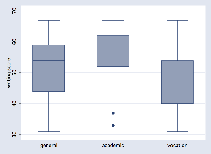
 graph box write, over(prog)
use http://www.philender.com/courses/data/hsb2, clear

tabulate write


    writing |
      score |      Freq.     Percent        Cum.
------------+-----------------------------------
         31 |          4        2.00        2.00
         33 |          4        2.00        4.00
         35 |          2        1.00        5.00
         36 |          2        1.00        6.00
         37 |          3        1.50        7.50
         38 |          1        0.50        8.00
         39 |          5        2.50       10.50
         40 |          3        1.50       12.00
         41 |         10        5.00       17.00
         42 |          2        1.00       18.00
         43 |          1        0.50       18.50
         44 |         12        6.00       24.50
         45 |          1        0.50       25.00
         46 |          9        4.50       29.50
         47 |          2        1.00       30.50
         49 |         11        5.50       36.00
         50 |          2        1.00       37.00
         52 |         15        7.50       44.50
         53 |          1        0.50       45.00
         54 |         17        8.50       53.50
         55 |          3        1.50       55.00
         57 |         12        6.00       61.00
         59 |         25       12.50       73.50
         60 |          4        2.00       75.50
         61 |          4        2.00       77.50
         62 |         18        9.00       86.50
         63 |          4        2.00       88.50
         65 |         16        8.00       96.50
         67 |          7        3.50      100.00
------------+-----------------------------------
      Total |        200      100.00
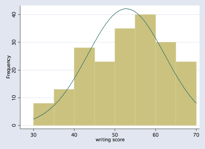
histogram write, start(30) width(5) freq normal
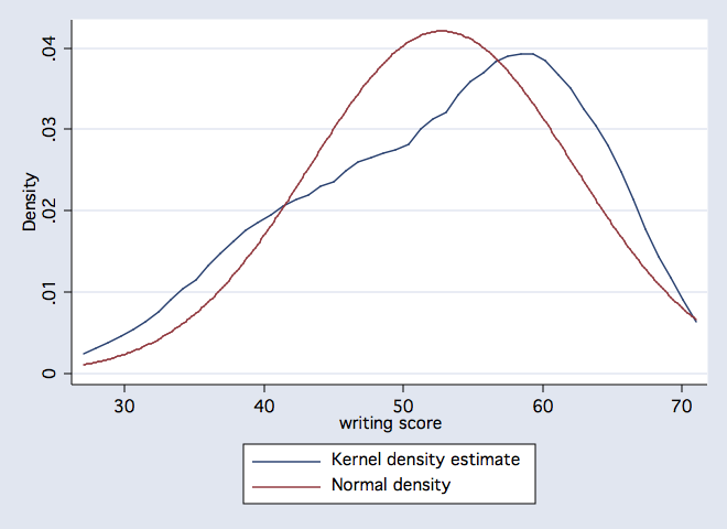
kdensity write, normal width(4)
stem write, lines(2)

Stem-and-leaf plot for write (writing score)

  3* | 11113333
  3. | 5566777899999
  4* | 0001111111111223444444444444
  4. | 56666666667799999999999
  5* | 00222222222222222344444444444444444
  5. | 5557777777777779999999999999999999999999
  6* | 000011112222222222222222223333
  6. | 55555555555555557777777

stem write, lines(5)

Stem-and-leaf plot for write (writing score)

  3* | 1111
  3t | 3333
  3f | 55
  3s | 66777
  3. | 899999
  4* | 0001111111111
  4t | 223
  4f | 4444444444445
  4s | 66666666677
  4. | 99999999999
  5* | 00
  5t | 2222222222222223
  5f | 44444444444444444555
  5s | 777777777777
  5. | 9999999999999999999999999
  6* | 00001111
  6t | 2222222222222222223333
  6f | 5555555555555555
  6s | 7777777
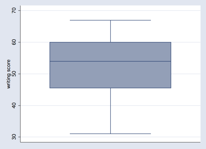
graph box write
summarize write, d
gen f=43 /* set value a little larger than highest freq bin */
gen pmin=r(min)
gen p25=r(p25)
gen p50=r(p50)
gen p75=r(p75)
gen pmax=r(max)
gen pmean=r(mean)
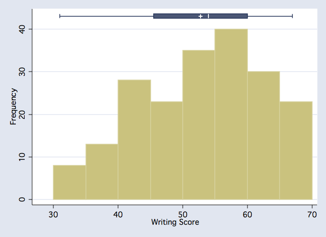
two (histogram write, start(30) width(5) freq) ///
(rcap pmin pmax f in 1, hor bcolor(dknavy)) ///
(rbar p25 p75 f in 1, hor bcolor(dknavy)) ///
(rcap p50 p50 f in 1, hor bcolor(white)) ///
(rcapsym pmean pmean f in 1, hor msym(plus) mcolor(white)), ///
legend(off) xtitle("Writing Score") ytitle("Frequency")
drop f-pmean
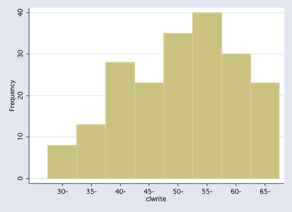
egen clwrite = cut(write), at(30(5)70) label

tabulate clwrite

    clwrite |      Freq.     Percent        Cum.
------------+-----------------------------------
        30- |          8        4.00        4.00
        35- |         13        6.50       10.50
        40- |         28       14.00       24.50
        45- |         23       11.50       36.00
        50- |         35       17.50       53.50
        55- |         40       20.00       73.50
        60- |         30       15.00       88.50
        65- |         23       11.50      100.00
------------+-----------------------------------
      Total |        200      100.00

codebook clwrite

------------------------------------------------------------------------------------------------------
clwrite                                                                                    (unlabeled)
------------------------------------------------------------------------------------------------------

                  type:  numeric (float)

                 range:  [30,65]                      units:  1
         unique values:  8                        missing .:  0/200

            tabulation:  Freq.  Value
                             8  30
                            13  35
                            28  40
                            23  45
                            35  50
                            40  55
                            30  60
                            23  65


histogram clwrite, freq discrete xlabel(0 "30-" 1 "35-" 2 "40-" 3 "45-" 4 "50-" 5 "55-" 6 "60-" 7  "65-")
Intro Home Page
Phil Ender, 13Oct99