In our section on t-tests we looked into testing the differences between two groups. One-way analysis of variance (ANOVA) allows us to investigate differences between more than two groups. We could have a single control groups and several different experimental groups. A one-way ANOVA has one independent variable with three or more levels.
Consider the following four group experiment:
Sources of Variability
The F-ratio
Hypotheses
Assumptions
| 1. | Independence |
| 2. | Normality |
| 3. | Homogeneity of Variance |
Example Four Group Problem
Level a1
a2 a3 a4 Total
3
6
3
3
2
2
2
1
3
4
5
4
4
2
3
3
7
6
8
7
6
6
5
5
8
7
9
8
11
9
10
10
Mean 2.75
3.5 6.25 9.0 5.375
Variance 2.214 0.857 1.071 1.714
ANOVA Summary Table
| Source | SS | df | MS | F | |
| Between Groups | 194.5 | 3 | 64.833 | 44.28 | |
| Within Groups | 41.0 | 28 | 1.464 | ||
| Total | 235.5 | 31 |
Homogeneity of Variance
Many textbooks show the use of the F-max test for verifying the assumption concerning homogeneity of variance. As you have been made aware the F-max test and other tests of homogeneity of variance are strongly influenced by nonnormality. The results can easily indicate heterogeneity of variance in situations where it is really not a problem. I recommend that you inspect the variances or standard deviations.
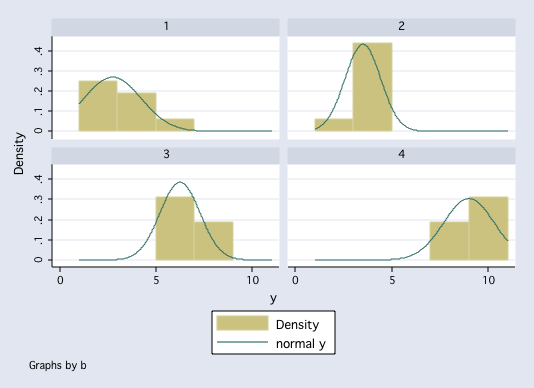
Normality
While checking the assumptions, you should inspect the histograms, for each of the groups, for normality. The cellgr command, available for ATS, makes the task very simple.
A Measure of Strength of Association
From the Example:
use http://www.philender.com/courses/data/crf24, clear

sort b a

by b: generate order = _n  /* create order for table below */

tabdisp order b, cellvar(y)

----------+-----------------------
          |           b
    order |    1     2     3     4
----------+-----------------------
        1 |    3     3     7     8
        2 |    6     4     6     7
        3 |    3     5     8     9
        4 |    3     4     7     8
        5 |    2     4     6    11
        6 |    2     2     6     9
        7 |    2     3     5    10
        8 |    1     3     5    10
----------+-----------------------

tabulate b, summarize(y)

            |            Summary of y
          b |        Mean   Std. Dev.       Freq.
------------+------------------------------------
          1 |        2.75   1.4880476           8
          2 |         3.5    .9258201           8
          3 |        6.25   1.0350983           8
          4 |           9   1.3093073           8
------------+------------------------------------
      Total |       5.375   2.7562246          32

histogram y, by(b) normal


anova y b

                     Number of obs =      32     R-squared     =  0.8259
                     Root MSE      = 1.21008     Adj R-squared =  0.8072

            Source |  Partial SS    df       MS           F     Prob > F
        -----------+----------------------------------------------------
             Model |      194.50     3  64.8333333      44.28     0.0000
                   |
                 b |      194.50     3  64.8333333      44.28     0.0000
                   |
          Residual |       41.00    28  1.46428571
        -----------+----------------------------------------------------
             Total |      235.50    31  7.59677419

omega2  /* Available from ATS via Internet */

 omega squared = 0.8023
 effect size   = 2.0142
anova y b
Number of obs = 32 R-squared = 0.8259
Root MSE = 1.21008 Adj R-squared = 0.8072
Source | Partial SS df MS F Prob > F
-----------+----------------------------------------------------
Model | 194.50 3 64.8333333 44.28 0.0000
|
b | 194.50 3 64.8333333 44.28 0.0000
|
Residual | 41.00 28 1.46428571
-----------+----------------------------------------------------
Total | 235.50 31 7.59677419
omega2 /* Available from ATS via Internet */
omega squared = 0.8023
effect size = 2.0142
Intro Home Page
Phil Ender, 22Nov00