
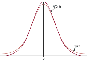
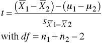
Use the Student's t Distribution.
The t-distribution is used to test groups differences when samples are small or when the population variance is unknown. The t-distribution is a family of curves that are symmetric and appear similar to the normal distribution, in fact, for extremely large samples the t and the normal distributions are identical. This is why statisticians say that the t-distribution is asymptotically normal. The t-distribution was first described by a British statistician named W.S. Gossett who worked for the Guinness Brewery in Dublin, Ireland. He published his results under the nom de plume of Student.
Each member of the family of curves in the t-distribution is a function of a parameter called the degrees of freedom. The t-distribution could be tabled in the same way that the normal distribution is, except that it would require a separate table for each of the curves. The t-distribution is tabled with several different probability levels as columns and degrees of freedom as rows. As part of the computation of the t-tests formulas, you will be given formulas the degrees of freedom.

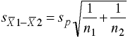
Where  is the standard error of the mean.
Is the class mean significantly different from the state mean?
First, compute the standard deviation from the variance:
s = SQRT(s2) = SQRT(121) =
11
Next, compute the standard error of the mean:
se = s/SQRT(n) = 11/SQRT(20) = 11/4.47 =
2.46
Compute the t-test:
t = (Xbar - μ)/se = (70.5 - 65)/2.46 = +2.24
The degrees of freedom, df = n -1 = 20 -1 = 19
The critical value for t at alpha = 0.05 is ±2.093
Thus, it is concluded that the class of third graders scored significantly higher than the state average.
| Control Group | Experimental Group |
|---|---|
| 102 | 107 |
| 99 | 125 |
| 90 | 111 |
| 121 | 117 |
| 114 | 122 |
Stata Examples
input group score x1
1 102  1
1  99  1
1  90  1
1 121  1
1 114  1
2 107 -1
2 125 -1
2 111 -1
2 117 -1
2 122 -1
end

ttest score, by(group)

Two-sample t test with equal variances

------------------------------------------------------------------------------
   Group |     Obs        Mean    Std. Err.   Std. Dev.   [95% Conf. Interval]
---------+--------------------------------------------------------------------
       1 |       5       105.2    5.508176    12.31666    89.90685    120.4931
       2 |       5       116.4    3.340659     7.46994    107.1248    125.6752
---------+--------------------------------------------------------------------
combined |      10       110.8    3.564641    11.27239    102.7362    118.8638
---------+--------------------------------------------------------------------
    diff |               -11.2    6.442049               -26.05539    3.655392
------------------------------------------------------------------------------
Degrees of freedom: 8

                      Ho: mean(1) - mean(2) = diff = 0

     Ha: diff < 0               Ha: diff ~= 0              Ha: diff > 0
       t =  -1.7386                t =  -1.7386              t =  -1.7386
   P < t =   0.0602          P > |t| =   0.1203          P > t =   0.9398

ttest score, by(group) unequal

Two-sample t test with unequal variances

------------------------------------------------------------------------------
   Group |     Obs        Mean    Std. Err.   Std. Dev.   [95% Conf. Interval]
---------+--------------------------------------------------------------------
       1 |       5       105.2    5.508176    12.31666    89.90685    120.4931
       2 |       5       116.4    3.340659     7.46994    107.1248    125.6752
---------+--------------------------------------------------------------------
combined |      10       110.8    3.564641    11.27239    102.7362    118.8638
---------+--------------------------------------------------------------------
    diff |               -11.2    6.442049               -26.62627    4.226274
------------------------------------------------------------------------------
Satterthwaite's degrees of freedom:  6.59196

                      Ho: mean(1) - mean(2) = diff = 0

     Ha: diff < 0               Ha: diff ~= 0              Ha: diff > 0
       t =  -1.7386                t =  -1.7386              t =  -1.7386
   P < t =   0.0642          P > |t| =   0.1283          P > t =   0.9358


use http://www.philender.com/courses/data/hsb2, clear


ttest write, by(female)

Two-sample t test with equal variances

------------------------------------------------------------------------------
   Group |     Obs        Mean    Std. Err.   Std. Dev.   [95% Conf. Interval]
---------+--------------------------------------------------------------------
    male |      91    50.12088    1.080274    10.30516    47.97473    52.26703
  female |     109    54.99083    .7790686    8.133715    53.44658    56.53507
---------+--------------------------------------------------------------------
combined |     200      52.775    .6702372    9.478586    51.45332    54.09668
---------+--------------------------------------------------------------------
    diff |           -4.869947    1.304191               -7.441835   -2.298059
------------------------------------------------------------------------------
Degrees of freedom: 198

                  Ho: mean(male) - mean(female) = diff = 0

     Ha: diff < 0               Ha: diff ~= 0              Ha: diff > 0
       t =  -3.7341                t =  -3.7341              t =  -3.7341
   P < t =   0.0001          P > |t| =   0.0002          P > t =   0.9999

ttest read, by(female)

Two-sample t test with equal variances

------------------------------------------------------------------------------
   Group |     Obs        Mean    Std. Err.   Std. Dev.   [95% Conf. Interval]
---------+--------------------------------------------------------------------
    male |      91    52.82418    1.101403    10.50671    50.63605     55.0123
  female |     109    51.73394    .9633659    10.05783    49.82439     53.6435
---------+--------------------------------------------------------------------
combined |     200       52.23    .7249921    10.25294    50.80035    53.65965
---------+--------------------------------------------------------------------
    diff |            1.090231    1.457507               -1.783997    3.964459
------------------------------------------------------------------------------
Degrees of freedom: 198

                  Ho: mean(male) - mean(female) = diff = 0

     Ha: diff < 0               Ha: diff ~= 0              Ha: diff > 0
       t =   0.7480                t =   0.7480              t =   0.7480
   P < t =   0.7723          P > |t| =   0.4553          P > t =   0.2277
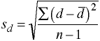

Degrees of freedom: df = n - 1, where n is the number of pairs of values.
| Wives | Husbands | d |
|---|---|---|
| 107 | 102 | 5 |
| 120 | 109 | 11 |
| 100 | 111 | -11 |
| 121 | 117 | 4 |
| 116 | 121 | -5 |
| 109 | 103 | 6 |
| 120 | 111 | 9 |
| 115 | 110 | 5 |
| 117 | 109 | 8 |
| 123 | 114 | 9 |
| 108 | 109 | -1 |
| 121 | 113 | 8 |
| mean | 4 |
input wife husb
107 102
120 109
100 111
121 117
116 121
109 103
120 111
115 110
117 109
123 114
108 109
121 113
end
generate diff = wife-husb
ttest wife=husb
Paired t test
------------------------------------------------------------------------------
Variable | Obs Mean Std. Err. Std. Dev. [95% Conf. Interval]
---------+--------------------------------------------------------------------
wife | 12 114.75 2.067516 7.162085 110.1994 119.3006
husb | 12 110.75 1.523179 5.276449 107.3975 114.1025
---------+--------------------------------------------------------------------
diff | 12 4 1.882938 6.522688 -.144318 8.144318
------------------------------------------------------------------------------
Ho: mean(wife - husb) = mean(diff) = 0
Ha: mean(diff) < 0 Ha: mean(diff) != 0 Ha: mean(diff) > 0
t = 2.1243 t = 2.1243 t = 2.1243
P < t = 0.9714 P > |t| = 0.0571 P > t = 0.0286
ttest diff=0
One-sample t test
------------------------------------------------------------------------------
Variable | Obs Mean Std. Err. Std. Dev. [95% Conf. Interval]
---------+--------------------------------------------------------------------
diff | 12 4 1.882938 6.522688 -.144318 8.144318
------------------------------------------------------------------------------
Degrees of freedom: 11
Ho: mean(diff) = 0
Ha: mean < 0 Ha: mean != 0 Ha: mean > 0
t = 2.1243 t = 2.1243 t = 2.1243
P < t = 0.9714 P > |t| = 0.0571 P > t = 0.0286
use http://www.philender.com/courses/data/hsb2, clear
generate diff = write - math
ttest write = math
Paired t test
------------------------------------------------------------------------------
Variable | Obs Mean Std. Err. Std. Dev. [95% Conf. Interval]
---------+--------------------------------------------------------------------
write | 200 52.775 .6702372 9.478586 51.45332 54.09668
math | 200 52.645 .6624493 9.368448 51.33868 53.95132
---------+--------------------------------------------------------------------
diff | 200 .13 .5828931 8.243353 -1.01944 1.27944
------------------------------------------------------------------------------
Ho: mean(write - math) = mean(diff) = 0
Ha: mean(diff) < 0 Ha: mean(diff) ~= 0 Ha: mean(diff) > 0
t = 0.2230 t = 0.2230 t = 0.2230
P < t = 0.5881 P > |t| = 0.8237 P > t = 0.4119
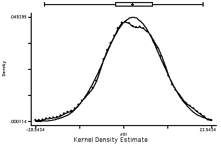
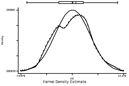
/* check normality of difference scores */
kdbox diff, norm mean /* findit kdbox */
 ttest write = math if female==1
Paired t test
------------------------------------------------------------------------------
Variable | Obs Mean Std. Err. Std. Dev. [95% Conf. Interval]
---------+--------------------------------------------------------------------
write | 109 54.99083 .7790686 8.133715 53.44658 56.53507
math | 109 52.3945 .8765083 9.151015 50.6571 54.13189
---------+--------------------------------------------------------------------
diff | 109 2.59633 .6734012 7.030515 1.261532 3.931128
------------------------------------------------------------------------------
Ho: mean(write - math) = mean(diff) = 0
Ha: mean(diff) < 0 Ha: mean(diff) ~= 0 Ha: mean(diff) > 0
t = 3.8555 t = 3.8555 t = 3.8555
P < t = 0.9999 P > |t| = 0.0002 P > t = 0.0001
/* check normality of difference scores */
kdbox diff if female==1, norm mean
ttest write = math if female==1
Paired t test
------------------------------------------------------------------------------
Variable | Obs Mean Std. Err. Std. Dev. [95% Conf. Interval]
---------+--------------------------------------------------------------------
write | 109 54.99083 .7790686 8.133715 53.44658 56.53507
math | 109 52.3945 .8765083 9.151015 50.6571 54.13189
---------+--------------------------------------------------------------------
diff | 109 2.59633 .6734012 7.030515 1.261532 3.931128
------------------------------------------------------------------------------
Ho: mean(write - math) = mean(diff) = 0
Ha: mean(diff) < 0 Ha: mean(diff) ~= 0 Ha: mean(diff) > 0
t = 3.8555 t = 3.8555 t = 3.8555
P < t = 0.9999 P > |t| = 0.0002 P > t = 0.0001
/* check normality of difference scores */
kdbox diff if female==1, norm mean
     effect size   power=.8   power=.7   power=.6
small      (0.2)      393        309        245
medium     (0.5)       63         50         40
large      (0.8)       25         20         16
very large (1.1)       13         11          9
These are just some generally suggested sample sizes to give you an idea of the range of possible
sample sizes, more precise estimates should be made for each individual study.
Intro Home Page
Phil Ender, 14Nov00