Scatterplots are used to plot two variables simultaneously, i.e., the joint distribution (also called a bivariate distribution) of two variables. Scatterplots that appear as a random circular cluster of points indicate low associations between the variables and would be said to have a a low degree of correlation (correlation close to zero). As the degree of association, and thus the correlation increases the circular cluster becomes more elliptical. The more narrow the ellipse the higher the correlation between the two variables and the higher the ability to predict one variable from another.
If the main axis of the ellipse slopes up to the right the assiciation is positive, if it slopes down to the right the association is negative. With positive correlations higher values on one variable are associated with heigher values on the other variable. When the correlation is negative, higher values on one variable are associated with lower values on the other.
Selected Scatter Plots
Pearson Product Moment Correlation Coefficient
Also known as, the Pearson correlation coefficient, or just the correlation coefficient.
Correlation coefficients can take on any value between -1 and +1, with ±1 representing perfect correlations between the variables. A correlation of zero represents no relationship between the variables.
A rule of thumb for interpreting correlation coefficients:
 Corr     Interpretation
 0 to .1  trivial
.1 to .3  small
.3 to .5  moderate
.5 to .7  large
.7 to .9  very large
Correlations are interpreted by squaring the value of the correlation coefficient. The squared value represents the proportion of variance of one variable that is shared with the other variable, in other words, the proportion of the variance of one variable that can be predicted from the other variable.
The squared correlation coefficient, r2, is know as the coefficient of determination. The proportion of variance that cannot be predicted or accounted for by the other variable is 1 - r2 and is also know as the coefficient of alienation.
Percent of Variance Accounted For
Correlation and Sample Size
The computation of correlation coefficients do not lend themselves to small sample sizes. The following table gives the recommended sample size for detecting various correlations with a power = 0.8 with an alpha = 0.05.
corr   n
.10   617
.20   153
.30    68
.40    37
.50    22
.60    15
.70    10
.80     7
.90     5
Covariance
Consider the variance as being the covariance of a variable with itself.
The Sample Correlation Coefficient
In deviation score form.
Calculator Computational Formula
Sources of Misleading Correlation Coefficients
Restriction of Range
Extreme Groups
Combining Groups
Outliers
Curvilinearity
Discuss Correlation & Causation
Of course, just because two variables are correlated it does not mean that they are causally related. Often a third variable, a lurking variable, that is not included in the analysis is responsible (causes) for the first two variables. A lurking variable is a variable that loiters in the background and affects both of the original variables
Stata Examples
use http://www.philender.com/courses/data/hsb2, clear
correlate female read write math science socst, cov
(obs=200)
| female read write math science socst
---------+------------------------------------------------------
female | .249221
read | -.271709 105.123
write | 1.21369 57.9967 89.8436
math | -.137211 63.6147 54.8293 87.7678
science | -.631407 63.9693 53.5339 58.5043 98.0276
socst | .280678 68.4089 61.5438 54.7626 49.4379 115.257
correlate female read write math science socst
(obs=200)
| female read write math science socst
---------+------------------------------------------------------
female | 1.0000
read | -0.0531 1.0000
write | 0.2565 0.5968 1.0000
math | -0.0293 0.6623 0.6174 1.0000
science | -0.1277 0.6302 0.5704 0.6307 1.0000
socst | 0.0524 0.6215 0.6048 0.5445 0.4651 1.0000
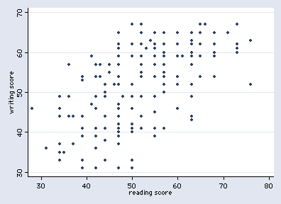
scatter write read
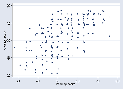
 scatter write read, jitter(2)
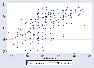
 twoway scatter write read, jitter(2) || lfit write read
 use http://www.philender.com/courses/data/hsb1, clear /* contains missing data */
pwcorr read write math science socst, obs star(.05)
| read write math science socst
----------+---------------------------------------------
read | 1.0000
| 200
|
write | 0.5968* 1.0000
| 200 200
|
math | 0.6623* 0.6174* 1.0000
| 200 200 200
|
science | 0.6171* 0.5671* 0.6166* 1.0000
| 195 195 195 195
|
socst | 0.6215* 0.6048* 0.5445* 0.4529* 1.0000
| 200 200 200 195 200
use http://www.philender.com/courses/data/hsb1, clear /* contains missing data */
pwcorr read write math science socst, obs star(.05)
| read write math science socst
----------+---------------------------------------------
read | 1.0000
| 200
|
write | 0.5968* 1.0000
| 200 200
|
math | 0.6623* 0.6174* 1.0000
| 200 200 200
|
science | 0.6171* 0.5671* 0.6166* 1.0000
| 195 195 195 195
|
socst | 0.6215* 0.6048* 0.5445* 0.4529* 1.0000
| 200 200 200 195 200
Intro Home Page
Phil Ender, 15Jan98