
Regression models involving proportions can present many of the same difficulties found with binary response variables. Proportions like binary variables have a minimum of zero and a maximum of one but unlike binary variables they also have values in between.
We can illustrate this with an OLS regression example. In the dataset proportion the variable meals is the proportion of free or reduced priced meals for each school.
OLS Proportion Example
use http://www.gseis.ucla.edu/courses/data/proportion
describe
Contains data from http://www.gseis.ucla.edu/courses/data/proportion.dta
obs: 4,421
vars: 6 24 Aug 2001 15:25
size: 75,157 (99.0% of memory free)
-------------------------------------------------------------------------------
storage display value
variable name type format label variable label
-------------------------------------------------------------------------------
api99 int %6.0g
meals float %4.0f pct free meals
ell byte %4.0f english language learners
yr_rnd byte %4.0f yr_rnd
parented float %9.0g avg parent ed
emer byte %4.0f pct emer credential
-------------------------------------------------------------------------------
summarize meals
Variable | Obs Mean Std. Dev. Min Max
-------------+-----------------------------------------------------
meals | 4421 .5188102 .3107313 0 1
graph meals, hist
 regress meals api99 ell parented
Source | SS df MS Number of obs = 4257
-------------+------------------------------ F( 3, 4253) = 7690.81
Model | 345.430324 3 115.143441 Prob > F = 0.0000
Residual | 63.6740571 4253 .014971563 R-squared = 0.8444
-------------+------------------------------ Adj R-squared = 0.8442
Total | 409.104381 4256 .09612415 Root MSE = .12236
------------------------------------------------------------------------------
meals | Coef. Std. Err. t P>|t| [95% Conf. Interval]
-------------+----------------------------------------------------------------
api99 | -.0011513 .0000277 -41.49 0.000 -.0012057 -.0010969
ell | .0027383 .0001238 22.11 0.000 .0024955 .0029811
parented | -.1133073 .0046346 -24.45 0.000 -.1223936 -.1042211
_cons | 1.489795 .0154935 96.16 0.000 1.459419 1.52017
------------------------------------------------------------------------------
predict preols
/* original response variable */
graph meals api99, ylab(0 1) yline(0 1)
regress meals api99 ell parented
Source | SS df MS Number of obs = 4257
-------------+------------------------------ F( 3, 4253) = 7690.81
Model | 345.430324 3 115.143441 Prob > F = 0.0000
Residual | 63.6740571 4253 .014971563 R-squared = 0.8444
-------------+------------------------------ Adj R-squared = 0.8442
Total | 409.104381 4256 .09612415 Root MSE = .12236
------------------------------------------------------------------------------
meals | Coef. Std. Err. t P>|t| [95% Conf. Interval]
-------------+----------------------------------------------------------------
api99 | -.0011513 .0000277 -41.49 0.000 -.0012057 -.0010969
ell | .0027383 .0001238 22.11 0.000 .0024955 .0029811
parented | -.1133073 .0046346 -24.45 0.000 -.1223936 -.1042211
_cons | 1.489795 .0154935 96.16 0.000 1.459419 1.52017
------------------------------------------------------------------------------
predict preols
/* original response variable */
graph meals api99, ylab(0 1) yline(0 1)
 /* predicted values from ols regression model */
graph preols api99, ylab(0 1) yline(0 1)
/* predicted values from ols regression model */
graph preols api99, ylab(0 1) yline(0 1)
One problem with this analysis is that some of the predicted proportions are less than zero or
greater than one. One solution to this situation is to use the logit transformation, ln(y/(1-y)). This is the same transformation that was used in logistic regression. There is one additional step, we will replace the zero and one values with .0001 and .9999 respectively in order to compute the log. Here is how the analysis with the logit transformation looks:
Logit Transformation
replace meals = .0001 if meals==0
replace meals = .9999 if meals==1

generate lmeals = ln(meals/(1-meals))

regress lmeals api99 ell parented

      Source |       SS       df       MS              Number of obs =    4257
-------------+------------------------------           F(  3,  4253) = 2533.98
       Model |  20573.8802     3  6857.96007           Prob > F      =  0.0000
    Residual |  11510.3287  4253  2.70640223           R-squared     =  0.6412
-------------+------------------------------           Adj R-squared =  0.6410
       Total |  32084.2089  4256  7.53858291           Root MSE      =  1.6451

------------------------------------------------------------------------------
      lmeals |      Coef.   Std. Err.      t    P>|t|     [95% Conf. Interval]
-------------+----------------------------------------------------------------
       api99 |  -.0082884   .0003731   -22.22   0.000    -.0090198    -.007557
         ell |    .027908   .0016651    16.76   0.000     .0246434    .0311725
    parented |  -.7978241   .0623126   -12.80   0.000    -.9199892    -.675659
       _cons |   7.035049   .2083104    33.77   0.000     6.626652    7.443446
------------------------------------------------------------------------------

predict plgt

summarize meals plgt

    Variable |     Obs        Mean   Std. Dev.       Min        Max
-------------+-----------------------------------------------------
       meals |    4421    .5188072   .3107231      .0001      .9999
        plgt |    4257    .2826891   2.198656  -4.647042   5.897199
As you can see, meals and plgt have very different means, standard deviations and
ranges. In order to get the predicted values scaled the same as the original variable, meals,
it is necessary to do a back or inverse transformation, in this case, 1/(1 + exp(-x)).
/* transform back to the same scale as meals */
generate premeals = 1/(1+exp(-plgt))

summarize meals premeals

    Variable |     Obs        Mean   Std. Dev.       Min        Max
-------------+-----------------------------------------------------
       meals |    4421    .5188072   .3107231      .0001      .9999
    premeals |    4257    .5304854   .3396622   .0094988   .9972604

graph premeals api99, ylab(0 1) yline(0 1)


corr meals preols premeals

(obs=4257)

             |    meals   preols premeals
-------------+---------------------------
       meals |   1.0000
      preols |   0.9189   1.0000
    premeals |   0.9226   0.9740   1.0000
corr meals preols premeals
(obs=4257)
| meals preols premeals
-------------+---------------------------
meals | 1.0000
preols | 0.9189 1.0000
premeals | 0.9226 0.9740 1.0000
The graph of the predicted values looks better than the OLS graph and the correlation between
meals and premeals is slightly larger than the correlation with preols. The
problem with all transformations is that the coefficients are given in terms of the transformed
variable. We need some additional tools to make the interpretation easier. GLM Approach
The above analysis worked out pretty good, but we were left with the transformed dependent variable which was more difficult to interpret than the original variable. GLM can be a tool to use in this situation. We will begin with a standard OLS type analysis followed by an alternative analysis using a logit link.
glm meals api99 ell parented, fam(gauss) link(ident)

Iteration 0:   log likelihood =  2904.6909

Generalized linear models                          No. of obs      =      4257
Optimization     : ML: Newton-Raphson              Residual df     =      4253
                                                   Scale parameter =  .0149716
Deviance         =  63.67405711                    (1/df) Deviance =  .0149716
Pearson          =  63.67405711                    (1/df) Pearson  =  .0149716

Variance function: V(u) = 1                        [Gaussian]
Link function    : g(u) = u                        [Identity]
Standard errors  : OIM

Log likelihood   =  2904.690914                    AIC             = -1.362786
BIC              = -35475.75476

------------------------------------------------------------------------------
       meals |      Coef.   Std. Err.      z    P>|z|     [95% Conf. Interval]
-------------+----------------------------------------------------------------
       api99 |  -.0011513   .0000277   -41.49   0.000    -.0012056   -.0010969
         ell |   .0027383   .0001238    22.11   0.000     .0024955     .002981
    parented |  -.1133073   .0046346   -24.45   0.000     -.122391   -.1042236
       _cons |   1.489795   .0154935    96.16   0.000     1.459428    1.520161
------------------------------------------------------------------------------
Note that this analysis is identical to the one using regress at the beginning of the unit.
Also note that the deviance is 63.67 and the BIC is -35475.75. Now, we will change the link
from identity to logit and run the analysis again.
glm meals api99 ell parented, fam(gauss) link(logit) nolog

Generalized linear models                          No. of obs      =      4257
Optimization     : ML: Newton-Raphson              Residual df     =      4253
                                                   Scale parameter =  .0135357
Deviance         =  57.56726076                    (1/df) Deviance =  .0135357
Pearson          =  57.56726076                    (1/df) Pearson  =  .0135357

Variance function: V(u) = 1                        [Gaussian]
Link function    : g(u) = ln(u/(1-u))              [Logit]
Standard errors  : OIM

Log likelihood   =  3119.293087                    AIC             =  -1.46361
BIC              = -35481.86155

------------------------------------------------------------------------------
       meals |      Coef.   Std. Err.      z    P>|z|     [95% Conf. Interval]
-------------+----------------------------------------------------------------
       api99 |  -.0057133   .0001431   -39.93   0.000    -.0059937   -.0054328
         ell |   .0172844   .0007045    24.54   0.000     .0159037    .0186651
    parented |   -.637455   .0242779   -26.26   0.000    -.6850389   -.5898711
       _cons |   5.079157   .0877114    57.91   0.000     4.907245    5.251068
------------------------------------------------------------------------------

glm, eform nohead

------------------------------------------------------------------------------
       meals |       ExpB   Std. Err.      z    P>|z|     [95% Conf. Interval]
-------------+----------------------------------------------------------------
       api99 |    .994303   .0001423   -39.93   0.000     .9940242    .9945819
         ell |   1.017435   .0007167    24.54   0.000     1.016031     1.01884
    parented |   .5286361   .0128342   -26.26   0.000     .5040706    .5543988
------------------------------------------------------------------------------

predict mu, mu

scatter mu api99, ylab(0 1) yline(0 1)
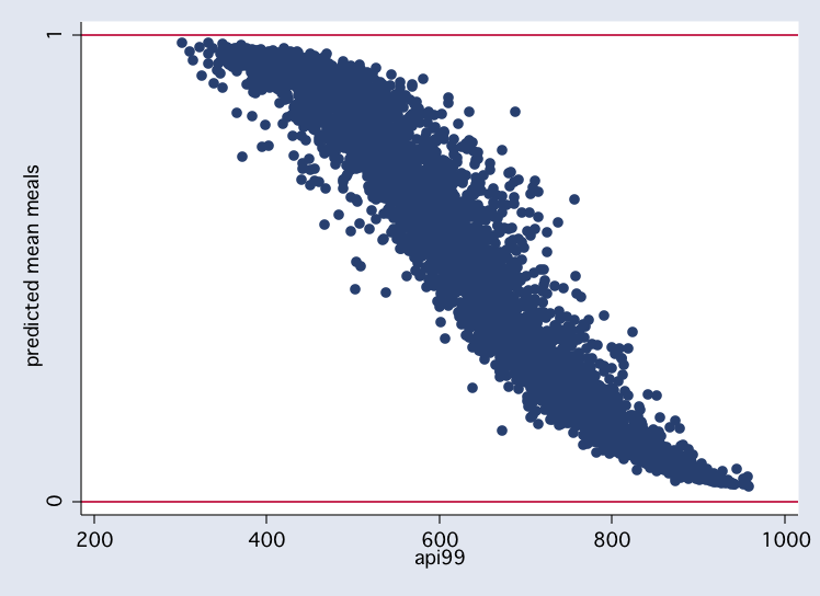
In this last analysis the deviance is reduced to 57.57 and the BIC has gone down to -35481.86, a
reduction of 6.11(which is non-trivial).Recent change to Stata allow users to run the model using the binomial family. Be sure to include the robust option to obtain the correct standard errors.
glm meals api99 ell parented, fam(binomial) link(logit) robust nolog

note: meals has non-integer values

Generalized linear models                          No. of obs      =      4257
Optimization     : ML: Newton-Raphson              Residual df     =      4253
                                                   Scale parameter =         1
Deviance         =  7347.932063                    (1/df) Deviance =  1.727706
Pearson          =  338.1971266                    (1/df) Pearson  =  .0795197

Variance function: V(u) = u*(1-u)                  [Bernoulli]
Link function    : g(u) = ln(u/(1-u))              [Logit]
Standard errors  : Sandwich

Log pseudo-likelihood = -1511.668612               AIC             =   .712083
BIC                   =-28191.49675

------------------------------------------------------------------------------
             |               Robust
       meals |      Coef.   Std. Err.      z    P>|z|     [95% Conf. Interval]
-------------+----------------------------------------------------------------
       api99 |  -.0058875   .0002051   -28.70   0.000    -.0062895   -.0054855
         ell |   .0167279   .0008299    20.16   0.000     .0151014    .0183545
    parented |  -.6575308   .0341978   -19.23   0.000    -.7245573   -.5905043
       _cons |   5.238212   .1015516    51.58   0.000     5.039174    5.437249
------------------------------------------------------------------------------

predict mu2, mu2

corr mu mu2
(obs=4257)

             |       mu      mu2
-------------+------------------
          mu |   1.0000
         mu2 |   1.0000   1.0000


label variable mu "mu"
label variable mu2 "mu2"

scatter mu mu2 api99, ylab(0 1) yline(0 1)
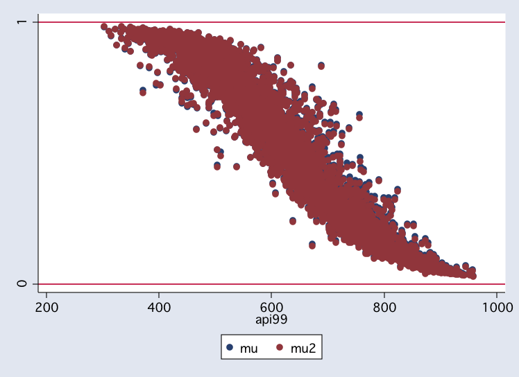
The deviance is very differnt from the previous models and the BIC actually appears to be larger.
However, the plots of the predicted values are virtuall identical, leading me to belive that
there is not much difference between the model using binomial and the model using gauss
for this set of data.
Categorical Data Analysis Course
Phil Ender -- revised 8/4/04