
Cox Proportional Hazards Model
Survival analysis is a very active field of investigation at this time. There are many different parametric estimation models. In these parametric methods the researcher specifies the probability distribution of the baseline hazard function. Using parametric survival analysis involves detailed knowledge of the likely distribution of the survival time. The Cox proportional hazard model, considered a semiparametric method, does not require the same detailed of knowledge about the distribution of the hazard function and is therefore a safer choice when there is no clear choice concerning the hazard function. There are many different parametric models and their use is beyond the scope of this course.
The following is a regression model for the hazard function
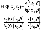
Under this model, the ratio of the hazard functions for two subjects with differing covartiate values is


use http://www.gseis.ucla.edu/courses/data/hivdata

stset time, failure(died)

     failure event:  died ~= 0 & died ~= .
obs. time interval:  (0, time]
 exit on or before:  failure

------------------------------------------------------------------------------
      100  total obs.
        0  exclusions
------------------------------------------------------------------------------
      100  obs. remaining, representing
       80  failures in single record/single failure data
     1136  total analysis time at risk, at risk from t =         0
                             earliest observed entry t =         0
                                  last observed exit t =        60

stcox drug age

         failure _d:  died
   analysis time _t:  time

Iteration 0:   log likelihood = -299.19502
Iteration 1:   log likelihood = -281.73399
Iteration 2:   log likelihood = -281.70404
Iteration 3:   log likelihood = -281.70404
Refining estimates:
Iteration 0:   log likelihood = -281.70404

Cox regression -- Breslow method for ties

No. of subjects =          100                     Number of obs   =       100
No. of failures =           80
Time at risk    =         1136
                                                   LR chi2(2)      =     34.98
Log likelihood  =   -281.70404                     Prob > chi2     =    0.0000

------------------------------------------------------------------------------
      _t |
      _d | Haz. Ratio   Std. Err.       z     P>|z|       [95% Conf. Interval]
---------+--------------------------------------------------------------------
    drug |   2.563531   .6550089      3.684   0.000        1.55363    4.229893
     age |   1.095852     .02026      4.951   0.000       1.056854    1.136289
------------------------------------------------------------------------------

stcox, nohr

Cox regression -- Breslow method for ties

No. of subjects =          100                     Number of obs   =       100
No. of failures =           80
Time at risk    =         1136
                                                   LR chi2(2)      =     34.98
Log likelihood  =   -281.70404                     Prob > chi2     =    0.0000

------------------------------------------------------------------------------
      _t |
      _d |      Coef.   Std. Err.       z     P>|z|       [95% Conf. Interval]
---------+--------------------------------------------------------------------
    drug |   .9413856   .2555104      3.684   0.000       .4405943    1.442177
     age |   .0915319   .0184879      4.951   0.000       .0552963    .1277675
------------------------------------------------------------------------------

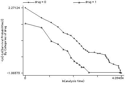
stphplot, by(drug)


 /* center age on median */
generate medage = age-35

stcox drug medage, nohr bases(b0)

Cox regression -- Breslow method for ties

No. of subjects =          100                     Number of obs   =       100
No. of failures =           80
Time at risk    =         1136
                                                   LR chi2(2)      =     34.98
Log likelihood  =   -281.70404                     Prob > chi2     =    0.0000

------------------------------------------------------------------------------
          _t |
          _d |      Coef.   Std. Err.      z    P>|z|     [95% Conf. Interval]
-------------+----------------------------------------------------------------
        drug |   .9413856   .2555104     3.68   0.000     .4405943    1.442177
      medage |   .0915319   .0184879     4.95   0.000     .0552963    .1277675
------------------------------------------------------------------------------

generate b1 = b0^exp(.9413856)

 /*  apply values to correct observations */
generate b0a = b0 if drug==0
generate b1a = b1 if drug==1

label variable b0a "IV Drug Use Absent"
label variable b1a "IV Drug Use Present"

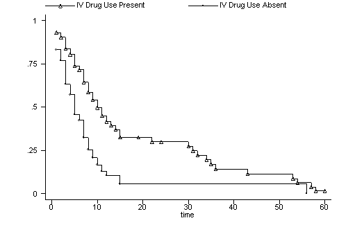
graph b0a b1a time, s(To) c(JJ) sort ylab(0 .25 to 1) xlab(0 10 to 60)

Testing the Proportional Hazards Assumption
The Cox model is appropriate only if the proportional hazards assumption holds. The proportional hazards assumption can be tested by testing the model specification. Below are three variations of tests of proportionality. With this example the three tests yielded consistent results, consistent results cannot be guarenteed to happen for all models.
Using linktest

stcox drug medage, nohr

(output omitted)

linktest

         failure _d:  died
   analysis time _t:  time

Cox regression -- Breslow method for ties

No. of subjects =          100                     Number of obs   =       100
No. of failures =           80
Time at risk    =         1136
                                                   LR chi2(2)      =     35.30
Log likelihood  =   -281.54467                     Prob > chi2     =    0.0000

------------------------------------------------------------------------------
          _t |
          _d |      Coef.   Std. Err.      z    P>|z|     [95% Conf. Interval]
-------------+----------------------------------------------------------------
        _hat |   1.102166   .2582422     4.27   0.000     .5960207    1.608312
      _hatsq |  -.0955469   .1721691    -0.55   0.579    -.4329922    .2418984
------------------------------------------------------------------------------

/* _hatsq not significant, supports proportionality */

Using the texp option

/* linear time */

stcox drug medage, tvc(drug medage) texp(_t) nohr

         failure _d:  died
   analysis time _t:  time

Cox regression -- Breslow method for ties

No. of subjects =          100                     Number of obs   =       100
No. of failures =           80
Time at risk    =         1136
                                                   LR chi2(4)      =     35.67
Log likelihood  =   -281.36147                     Prob > chi2     =    0.0000

------------------------------------------------------------------------------
          _t |
          _d |      Coef.   Std. Err.      z    P>|z|     [95% Conf. Interval]
-------------+----------------------------------------------------------------
rh           |
        drug |   1.128467    .355839     3.17   0.002     .4310356    1.825899
      medage |   .0909066   .0235272     3.86   0.000     .0447941     .137019
-------------+----------------------------------------------------------------
t            |
        drug |  -.0295158   .0403228    -0.73   0.464     -.108547    .0495154
      medage |  -.0001681   .0014418    -0.12   0.907    -.0029939    .0026578
------------------------------------------------------------------------------

note: second equation contains variables that continuously vary with respect to time; variables are interacted
      with current values of _t.

test [t]

 ( 1)  [t]drug = 0.0
 ( 2)  [t]medage = 0.0

           chi2(  2) =    0.54
         Prob > chi2 =    0.7616  /* not significant, supports proportionality */

/* log time */

stcox drug medage, tvc(drug medage) texp(ln(_t)) nohr

         failure _d:  died
   analysis time _t:  time

Cox regression -- Breslow method for ties

No. of subjects =          100                     Number of obs   =       100
No. of failures =           80
Time at risk    =         1136
                                                   LR chi2(4)      =     35.16
Log likelihood  =   -281.61464                     Prob > chi2     =    0.0000

------------------------------------------------------------------------------
          _t |
          _d |      Coef.   Std. Err.      z    P>|z|     [95% Conf. Interval]
-------------+----------------------------------------------------------------
rh           |
        drug |   .8916303   .4560034     1.96   0.051      -.00212     1.78538
      medage |   .0811645   .0309948     2.62   0.009     .0204159    .1419132
-------------+----------------------------------------------------------------
t            |
        drug |   .0401428    .267503     0.15   0.881    -.4841535    .5644391
      medage |   .0065743   .0156238     0.42   0.674    -.0240477    .0371964
------------------------------------------------------------------------------

note: second equation contains variables that continuously vary with respect to time;
      variables are interacted with current values of ln(_t).

test [t]

 ( 1)  [t]drug = 0.0
 ( 2)  [t]medage = 0.0

           chi2(  2) =    0.18
         Prob > chi2 =    0.9145  /* not significant, supports proportionality */

Test based on Schoenfeld residuals

stcox drug medage, schoenfeld(sch*) scaledsch(sca*) nohr

(output omitted)

stphtest

      Test of proportional hazards assumption

      Time:  Time
      ----------------------------------------------------------------
                  |                      chi2       df       Prob>chi2
      ------------+---------------------------------------------------
      global test |                      0.25        2         0.8824
      ----------------------------------------------------------------

  /* global test not significant, supports proportionality */
Categorical Data Analysis Course
Phil Ender