

In this unit we present an introduction to survival analysis, also known as event history analysis or time-to-event analysis in the social sciences. Analyses of this type involve the amount of time that a subject is at risk while under observation. Time, itself, can be measured in different ways, it can be continuous or it treated as discrete. In this unit we will look into continuous time survival analysis and in the next unit we will give an introduction to discrete time suvival analysis.
There are two aspects of survival analysis that make the it interesting from a data analysis perspective are:
In some studies, all of the cases might be observed until failure or the specific event occurs. In other studies, the study may end before failure occurs for some subjects or some subjects may withdraw or dropout of the study before the failure event. In either event, the subject is not under observation when the failure occurs. When a subject is not observed until failure, the observation is considered to be censored. These types of right censored data are common in survival analysis. At times, analyses might also include left censored data.
Suvivorship and Hazard Functions
Let the probability density function and and cumulative density funtion be denoted as follows:
Now, we can define the survivorship function as:
The hazard function can next be defined as:
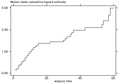
However, it is probably easier to interpret the cumulative hazard function, H(t), which is just the integral over 0 to t of h(t).
Stata survival time commands, such as, sts list and sts graph can display results in either the survivorship or hazard metric.
Nonparametric Methods
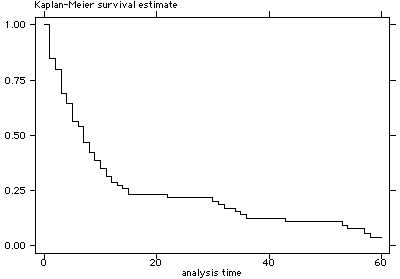
There are two nonparametric approaches commonly used to estimate the survivor function and cumulative hazard function. The Kaplan-Meier (1958) method estimates the survivor function and the Nelson-Aalen (1972 & 1978) method estimates the cumulative hazard function. These nonparametric estimators require only an ordering of the time to failure (or censoring) and do not include the effects of covariates. We will begin our explanation of the Kaplan-Meier estimator with the following simple example.
id t failed
1  2   1
2  4   1
3  4   1
4  5   0
5  7   1
6  8   0
We can summarize the data as follows:
              nj            dj
at time    # at risk    # failed    # censored
  2           6             1            0
  4           5             2            0
  5           3             0            1
  7           2             1            0
  8           1             0            1
Using the formula,

we can compute a probability column and also the continuous product of the probabilities.
              nj            dj
at time    # at risk    # failed    # censored    p     S(t)
  2           6             1            0       5/6     5/6
  4           5             2            0       3/5     1/2
  5           3             0            1        1      1/2
  7           2             1            0       1/2     1/4
  8           1             0            1        1      1/4
The last column contains the Kaplan-Meier survivor function.
In Stata, we would use the sts list command to obtain the Kaplan-Meier survivor function. Before we can use the sts list command we need to get the data into the proper format for survival analysis by using the stset command. Here is how it is done in Stata.
input id t failed
1  2   1
2  4   1
3  4   1
4  5   0
5  7   1
6  8   0
end

stset t, failure(failed)

     failure event:  failed ~= 0 & failed ~= .
obs. time interval:  (0, t]
 exit on or before:  failure

------------------------------------------------------------------------------
        6  total obs.
        0  exclusions
------------------------------------------------------------------------------
        6  obs. remaining, representing
        4  failures in single record/single failure data
       30  total analysis time at risk, at risk from t =         0
                             earliest observed entry t =         0
                                  last observed exit t =         8

sts list

         failure _d:  failed
   analysis time _t:  t

           Beg.          Net            Survivor      Std.
  Time    Total   Fail   Lost           Function     Error     [95% Conf. Int.]
-------------------------------------------------------------------------------
     2        6      1      0             0.8333    0.1521     0.2731    0.9747
     4        5      2      0             0.5000    0.2041     0.1109    0.8037
     5        3      0      1             0.5000    0.2041     0.1109    0.8037
     7        2      1      0             0.2500    0.2041     0.0123    0.6459
     8        1      0      1             0.2500    0.2041     0.0123    0.6459
-------------------------------------------------------------------------------
You might think that it would be easy to obtain the cumulative hazard function from
the Kaplan-Meier using the relatioship between the survivor and hazard functions (see above) but
there are problems in small samples with this approach. It is better to use the following
formula for the Nelson-Aalen estimator.

We will compute the column ej = dj/nj and the column H(t) which is the sum of the ej.
              nj            dj
at time    # at risk    # failed    # censored    ej      H(t)
  2           6             1            0       1/6    0.1667
  4           5             2            0       2/5    0.5667
  5           3             0            1        0     0.5667
  7           2             1            0       1/2    1.0667
  8           1             0            1        0     1.0667
In Stata, we use the na option with sts list.
sts list, na

         failure _d:  failed
   analysis time _t:  t

           Beg.          Net          Nelson-Aalen    Std.
  Time    Total   Fail   Lost           Cum. Haz.    Error     [95% Conf. Int.]
-------------------------------------------------------------------------------
     2        6      1      0             0.1667    0.1667     0.0235    1.1832
     4        5      2      0             0.5667    0.3283     0.1820    1.7639
     5        3      0      1             0.5667    0.3283     0.1820    1.7639
     7        2      1      0             1.0667    0.5981     0.3554    3.2015
     8        1      0      1             1.0667    0.5981     0.3554    3.2015
-------------------------------------------------------------------------------
Note: Due to the introductory nature of this unit we do go into issues such as delayed entry, interval truncation, interval censoring, etc.
HIV Example
Here is an example using HIV data from Hosmer & Lemeshow (1999).
use http://www.gseis.ucla.edu/courses/data/hivdata
describe
Contains data from http://www.gseis.ucla.edu/courses/data/hivdata.dta
obs: 100
vars: 7 7 Feb 2001 02:07
size: 3,800 (99.5% of memory free)
-------------------------------------------------------------------------------
storage display value
variable name type format label variable label
-------------------------------------------------------------------------------
id float %9.0g
entdate str7 %9s
enddate str7 %9s
time float %9.0g
age float %9.0g
drug float %9.0g
died float %9.0g
-------------------------------------------------------------------------------
list entdate enddate time died in 1/15
entdate enddate time died
1. 15may90 14oct90 5 1
2. 19sep89 20mar90 6 0
3. 21apr91 20dec91 8 1
4. 03jan91 04apr91 3 1
5. 18sep89 19jul91 22 1
6. 18mar91 17apr91 1 0
7. 11nov89 11jun90 7 1
8. 25nov89 25aug90 9 1
9. 11feb91 13may91 3 1
10. 11aug89 11aug90 12 1
11. 11apr90 10jun90 2 0
12. 11may91 10may92 12 1
13. 17jan89 16feb89 1 1
14. 16feb91 17may92 15 1
15. 09apr91 06feb94 34 1
list time died drug age in 1/15
time died drug age
1. 5 1 0 46
2. 6 0 1 35
3. 8 1 1 30
4. 3 1 1 30
5. 22 1 0 36
6. 1 0 1 32
7. 7 1 1 36
8. 9 1 1 31
9. 3 1 0 48
10. 12 1 0 47
11. 2 0 1 28
12. 12 1 0 34
13. 1 1 1 44
14. 15 1 1 32
15. 34 1 0 36
summarize
Variable | Obs Mean Std. Dev. Min Max
---------+-----------------------------------------------------
id | 100 50.5 29.01149 1 100
entdate | 0
enddate | 0
time | 100 11.36 15.28353 1 60
age | 100 36.07 6.700302 20 54
drug | 100 .49 .5024184 0 1
died | 100 .8 .4020151 0 1
tab1 drug age
-> tabulation of drug
drug | Freq. Percent Cum.
------------+-----------------------------------
0 | 51 51.00 51.00
1 | 49 49.00 100.00
------------+-----------------------------------
Total | 100 100.00
-> tabulation of age
age | Freq. Percent Cum.
------------+-----------------------------------
20 | 1 1.00 1.00
21 | 1 1.00 2.00
22 | 1 1.00 3.00
25 | 2 2.00 5.00
26 | 2 2.00 7.00
28 | 3 3.00 10.00
29 | 2 2.00 12.00
30 | 6 6.00 18.00
31 | 5 5.00 23.00
32 | 9 9.00 32.00
33 | 6 6.00 38.00
34 | 8 8.00 46.00
35 | 5 5.00 51.00
36 | 9 9.00 60.00
37 | 3 3.00 63.00
38 | 3 3.00 66.00
39 | 5 5.00 71.00
40 | 3 3.00 74.00
41 | 4 4.00 78.00
42 | 4 4.00 82.00
43 | 2 2.00 84.00
44 | 4 4.00 88.00
45 | 1 1.00 89.00
46 | 3 3.00 92.00
47 | 4 4.00 96.00
48 | 1 1.00 97.00
50 | 1 1.00 98.00
51 | 1 1.00 99.00
54 | 1 1.00 100.00
------------+-----------------------------------
Total | 100 100.00
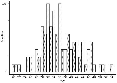
hist age
 stset time, failure(died)
failure event: died ~= 0 & died ~= .
obs. time interval: (0, time]
exit on or before: failure
------------------------------------------------------------------------------
100 total obs.
0 exclusions
------------------------------------------------------------------------------
100 obs. remaining, representing
80 failures in single record/single failure data
1136 total analysis time at risk, at risk from t = 0
earliest observed entry t = 0
last observed exit t = 60
list id _st- _t0 in 1/20
id _st _d _t _t0
1. 1 1 1 5 0
2. 2 1 0 6 0
3. 3 1 1 8 0
4. 4 1 1 3 0
5. 5 1 1 22 0
6. 6 1 0 1 0
7. 7 1 1 7 0
8. 8 1 1 9 0
9. 9 1 1 3 0
10. 10 1 1 12 0
11. 11 1 0 2 0
12. 12 1 1 12 0
13. 13 1 1 1 0
14. 14 1 1 15 0
15. 15 1 1 34 0
16. 16 1 1 1 0
17. 17 1 1 4 0
18. 18 1 0 19 0
19. 19 1 0 3 0
20. 20 1 1 2 0
stdes
failure _d: died
analysis time _t: time
|-------------- per subject --------------|
Category total mean min median max
------------------------------------------------------------------------------
no. of subjects 100
no. of records 100 1 1 1 1
(first) entry time 0 0 0 0
(final) exit time 11.36 1 5 60
subjects with gap 0
time on gap if gap 0
time at risk 1136 11.36 1 5 60
failures 80 .8 0 1 1
------------------------------------------------------------------------------
stvary
failure _d: died
analysis time _t: time
subjects for whom the variable is
never always sometimes
variable | constant varying missing missing missing
---------+--------------------------------------------------------------
id | 100 0 100 0 0
entdate | 100 0 100 0 0
enddate | 100 0 100 0 0
age | 100 0 100 0 0
drug | 100 0 100 0 0
stsum
failure _d: died
analysis time _t: time
| incidence no. of |------ Survival time -----|
| time at risk rate subjects 25% 50% 75%
---------+---------------------------------------------------------------------
total | 1136 .0704225 100 3 7 15
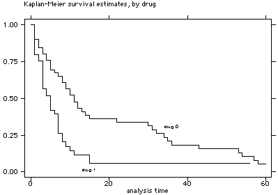
stsum, by(drug)
failure _d: died
analysis time _t: time
| incidence no. of |------ Survival time -----|
drug | time at risk rate subjects 25% 50% 75%
---------+---------------------------------------------------------------------
0 | 864 .0486111 51 5 11 34
1 | 272 .1397059 49 3 5 8
---------+---------------------------------------------------------------------
total | 1136 .0704225 100 3 7 15
sts list
failure _d: died
analysis time _t: time
Beg. Net Survivor Std.
Time Total Fail Lost Function Error [95% Conf. Int.]
-------------------------------------------------------------------------------
1 100 15 2 0.8500 0.0357 0.7636 0.9067
2 83 5 5 0.7988 0.0402 0.7057 0.8652
3 73 10 2 0.6894 0.0473 0.5862 0.7718
4 61 4 1 0.6442 0.0493 0.5387 0.7315
5 56 7 0 0.5636 0.0517 0.4564 0.6577
6 49 2 1 0.5406 0.0521 0.4334 0.6361
7 46 6 1 0.4701 0.0526 0.3644 0.5688
8 39 4 0 0.4219 0.0525 0.3183 0.5217
9 35 3 0 0.3857 0.0520 0.2845 0.4858
10 32 3 1 0.3496 0.0511 0.2514 0.4493
11 28 3 0 0.3121 0.0500 0.2177 0.4110
12 25 2 2 0.2872 0.0490 0.1956 0.3851
13 21 1 0 0.2735 0.0486 0.1835 0.3711
14 20 1 0 0.2598 0.0480 0.1715 0.3569
15 19 2 0 0.2325 0.0467 0.1479 0.3282
19 17 0 1 0.2325 0.0467 0.1479 0.3282
22 16 1 0 0.2179 0.0460 0.1355 0.3130
24 15 0 1 0.2179 0.0460 0.1355 0.3130
30 14 1 0 0.2024 0.0453 0.1222 0.2969
31 13 1 0 0.1868 0.0444 0.1092 0.2805
32 12 1 0 0.1712 0.0433 0.0966 0.2638
34 11 1 0 0.1557 0.0421 0.0843 0.2469
35 10 1 0 0.1401 0.0407 0.0724 0.2296
36 9 1 0 0.1245 0.0390 0.0610 0.2119
43 8 1 0 0.1090 0.0371 0.0500 0.1939
53 7 1 0 0.0934 0.0349 0.0396 0.1754
54 6 1 0 0.0778 0.0324 0.0298 0.1564
56 5 0 1 0.0778 0.0324 0.0298 0.1564
57 4 1 0 0.0584 0.0296 0.0178 0.1349
58 3 1 0 0.0389 0.0253 0.0082 0.1117
60 2 0 2 0.0389 0.0253 0.0082 0.1117
-------------------------------------------------------------------------------
sts list, by(drug) compare
failure _d: died
analysis time _t: time
Survivor Function
drug 0 1
----------------------------------
time 1 0.9020 0.7959
8 0.6078 0.2037
15 0.3624 0.0582
22 0.3383 0.0582
29 0.3383 0.0582
36 0.1821 0.0582
43 0.1561 0.0582
50 0.1561 0.0582
57 0.0781 .
64 . .
----------------------------------
sts graph
 sts graph, na
 sts graph, by(drug)
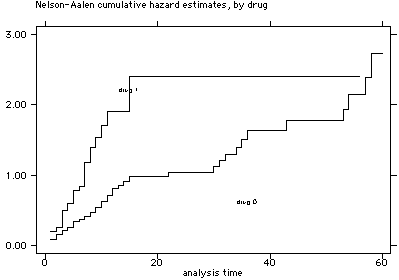
 sts graph, by(drug) na
Categorical Data Analysis Course
Phil Ender