
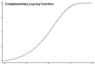
Complementary log-log models repesent a third altenative to logistic regression and probit analysis for binary response variables. Complementary log-log models are fequently used when the probability of an event is very small or very large. Unlike logit and probit the complementary log-log function is asymmetrical. A graph of the complementary log-log fuanction is given below.
Examples follow a similar pattern that the ones in logit and probit analyses.
Example 1
set matsize 100
use http://www.gseis.ucla.edu/courses/data/honors

tab ses, gen(ses)

        ses |      Freq.     Percent        Cum.
------------+-----------------------------------
        low |         47       23.50       23.50
     middle |         95       47.50       71.00
       high |         58       29.00      100.00
------------+-----------------------------------
      Total |        200      100.00


cloglog honors lang math female ses1 ses2

Complementary log-log regression                Number of obs     =        200
                                                Zero outcomes     =        147
                                                Nonzero outcomes  =         53

                                                LR chi2(5)        =      87.46
Log likelihood =  -71.91256                     Prob > chi2       =     0.0000

------------------------------------------------------------------------------
      honors |      Coef.   Std. Err.      z    P>|z|     [95% Conf. Interval]
-------------+----------------------------------------------------------------
        lang |   .0480773   .0213486     2.25   0.024     .0062348    .0899197
        math |   .1075815    .024252     4.44   0.000     .0600485    .1551145
      female |   .8893274    .332183     2.68   0.007     .2382606    1.540394
        ses1 |   .0151648   .4334635     0.03   0.972     -.834408    .8647376
        ses2 |  -.8427618    .357412    -2.36   0.018    -1.543276   -.1422472
       _cons |  -10.05438   1.401321    -7.17   0.000    -12.80092   -7.307837
------------------------------------------------------------------------------

listcoef

cloglog (N=200): Unstandardized and Standardized Estimates

 Observed SD: .4424407

-------------------------------------------------------------
      honors |      b         z     P>|z|    bStdX      SDofX
-------------+-----------------------------------------------
        lang |   0.04808    2.252   0.024   0.4929    10.2529
        math |   0.10758    4.436   0.000   1.0079     9.3684
      female |   0.88933    2.677   0.007   0.4440     0.4992
        ses1 |   0.01516    0.035   0.972   0.0064     0.4251
        ses2 |  -0.84276   -2.358   0.018  -0.4219     0.5006
-------------------------------------------------------------

prchange

cloglog: Changes in Predicted Probabilities for honors

        min->max      0->1     -+1/2    -+sd/2
  lang    0.3564    0.0007    0.0068    0.0699
  math    0.8223    0.0001    0.0152    0.1453
female    0.1235    0.1235    0.1276    0.0629
  ses1    0.0021    0.0021    0.0021    0.0009
  ses2   -0.1187   -0.1187   -0.1207   -0.0598

              0       1
Pr(y|x)  0.8465  0.1535

           lang     math   female     ses1     ses2
    x=    52.23   52.645     .545     .235     .475
sd(x)=  10.2529  9.36845   .49922  .425063  .500628

mfx compute

Marginal effects after cloglog
      y  = Pr(honors) (predict)
         =  .15352122
------------------------------------------------------------------------------
variable |      dy/dx    Std. Err.     z    P>|z|  [    95% C.I.   ]      X
---------+--------------------------------------------------------------------
    lang |   .0067829      .00301    2.26   0.024    .00089  .012675   52.2300
    math |   .0151779      .00338    4.49   0.000    .00855  .021806   52.6450
  female*|   .1234855        .046    2.68   0.007   .033327  .213644   .545000
    ses1*|   .0021467      .06156    0.03   0.972  -.118504  .122798   .235000
    ses2*|  -.1186566      .05132   -2.31   0.021  -.219241 -.018072   .475000
------------------------------------------------------------------------------
(*) dy/dx is for discrete change of dummy variable from 0 to 1


prtab math

cloglog: Predicted probabilities of positive outcome for honors

----------------------
math      |
score     | Prediction
----------+-----------
       33 |     0.0199
       35 |     0.0247
       37 |     0.0305
       38 |     0.0339
       39 |     0.0377
       40 |     0.0419
       41 |     0.0465
       42 |     0.0516
       43 |     0.0573
       44 |     0.0636
       45 |     0.0706
       46 |     0.0783
       47 |     0.0868
       48 |     0.0962
       49 |     0.1065
       50 |     0.1179
       51 |     0.1303
       52 |     0.1440
       53 |     0.1590
       54 |     0.1754
       55 |     0.1932
       56 |     0.2127
       57 |     0.2338
       58 |     0.2566
       59 |     0.2812
       60 |     0.3077
       61 |     0.3360
       62 |     0.3662
       63 |     0.3982
       64 |     0.4319
       65 |     0.4672
       66 |     0.5040
       67 |     0.5420
       68 |     0.5808
       69 |     0.6203
       70 |     0.6598
       71 |     0.6990
       72 |     0.7374
       73 |     0.7744
       75 |     0.8422
----------------------

      lang    math  female    ses1    ses2
x=   52.23  52.645    .545    .235    .475

prtab female

cloglog: Predicted probabilities of positive outcome for honors

----------------------
   female | Prediction
----------+-----------
     male |     0.0976
   female |     0.2210
----------------------

      lang    math  female    ses1    ses2
x=   52.23  52.645    .545    .235    .475

prtab math female

cloglog: Predicted probabilities of positive outcome for honors

--------------------------
math      |     female
score     |   male  female
----------+---------------
       33 | 0.0123  0.0297
       35 | 0.0153  0.0367
       37 | 0.0189  0.0454
       38 | 0.0210  0.0504
       39 | 0.0234  0.0559
       40 | 0.0260  0.0621
       41 | 0.0289  0.0689
       42 | 0.0321  0.0764
       43 | 0.0357  0.0847
       44 | 0.0397  0.0939
       45 | 0.0441  0.1039
       46 | 0.0490  0.1150
       47 | 0.0544  0.1272
       48 | 0.0604  0.1406
       49 | 0.0670  0.1553
       50 | 0.0743  0.1713
       51 | 0.0824  0.1888
       52 | 0.0913  0.2079
       53 | 0.1012  0.2286
       54 | 0.1120  0.2510
       55 | 0.1239  0.2752
       56 | 0.1369  0.3012
       57 | 0.1513  0.3291
       58 | 0.1669  0.3588
       59 | 0.1840  0.3904
       60 | 0.2027  0.4237
       61 | 0.2229  0.4587
       62 | 0.2448  0.4951
       63 | 0.2686  0.5328
       64 | 0.2941  0.5715
       65 | 0.3215  0.6108
       66 | 0.3507  0.6504
       67 | 0.3818  0.6897
       68 | 0.4146  0.7283
       69 | 0.4492  0.7657
       70 | 0.4853  0.8013
       71 | 0.5227  0.8346
       72 | 0.5611  0.8652
       73 | 0.6003  0.8926
       75 | 0.6793  0.9372
--------------------------

      lang    math  female    ses1    ses2
x=   52.23  52.645    .545    .235    .475


Example 2
use http://www.gseis.ucla.edu/courses/data/retain

describe

Contains data from http://www.gseis.ucla.edu/courses/data/retain.dta
  obs:           200
 vars:             6                          8 Feb 2001 13:20
 size:         5,600 (99.9% of memory free)
-------------------------------------------------------------------------------
              storage  display     value
variable name   type   format      label      variable label
-------------------------------------------------------------------------------
id              float  %9.0g
female          float  %9.0g       fl
read            float  %9.0g                  reading test
math            float  %9.0g                  math test
retain          float  %9.0g                  not promoted
work            float  %9.0g                  work 1/2 day
-------------------------------------------------------------------------------

summarize

    Variable |     Obs        Mean   Std. Dev.       Min        Max
-------------+-----------------------------------------------------
          id |     200       100.5   57.87918          1        200
      female |     200        .545   .4992205          0          1
        read |     200       52.23   10.25294         28         76
        math |     200      52.645   9.368448         33         75
      retain |     200        .045   .2078243          0          1
        work |     200         .26    .439735          0          1

tab1 female work retain

-> tabulation of female

     female |      Freq.     Percent        Cum.
------------+-----------------------------------
       male |         91       45.50       45.50
     female |        109       54.50      100.00
------------+-----------------------------------
      Total |        200      100.00

-> tabulation of work

   work 1/2 |
        day |      Freq.     Percent        Cum.
------------+-----------------------------------
          0 |        148       74.00       74.00
          1 |         52       26.00      100.00
------------+-----------------------------------
      Total |        200      100.00

-> tabulation of retain

        not |
   promoted |      Freq.     Percent        Cum.
------------+-----------------------------------
          0 |        191       95.50       95.50
          1 |          9        4.50      100.00
------------+-----------------------------------
      Total |        200      100.00

cloglog retain read math female work

Complementary log-log regression                Number of obs     =        200
                                                Zero outcomes     =        191
                                                Nonzero outcomes  =          9

                                                LR chi2(4)        =      21.54
Log likelihood = -25.936448                     Prob > chi2       =     0.0002

------------------------------------------------------------------------------
      retain |      Coef.   Std. Err.      z    P>|z|     [95% Conf. Interval]
-------------+----------------------------------------------------------------
        read |  -.0778436   .0470081    -1.66   0.098    -.1699778    .0142906
        math |   -.064375   .0595326    -1.08   0.280    -.1810567    .0523067
      female |  -2.396835   1.067861    -2.24   0.025    -4.489804   -.3038662
        work |   .7195881   .8009147     0.90   0.369    -.8501759    2.289352
       _cons |   4.075455   3.195718     1.28   0.202    -2.188038    10.33895
------------------------------------------------------------------------------

cloglog retain read female work

Complementary log-log regression                Number of obs     =        200
                                                Zero outcomes     =        191
                                                Nonzero outcomes  =          9

                                                LR chi2(3)        =      20.26
Log likelihood =  -26.57175                     Prob > chi2       =     0.0001

------------------------------------------------------------------------------
      retain |      Coef.   Std. Err.      z    P>|z|     [95% Conf. Interval]
-------------+----------------------------------------------------------------
        read |  -.0952269   .0448223    -2.12   0.034    -.1830769   -.0073769
      female |  -2.270178    1.06383    -2.13   0.033    -4.355246   -.1851093
        work |     .91947   .8013326     1.15   0.251     -.651113    2.490053
       _cons |   1.698534   2.215278     0.77   0.443    -2.643331    6.040398
------------------------------------------------------------------------------

linktest

Complementary log-log regression                Number of obs     =        200
                                                Zero outcomes     =        191
                                                Nonzero outcomes  =          9

                                                LR chi2(2)        =      32.25
Log likelihood = -20.578686                     Prob > chi2       =     0.0000

------------------------------------------------------------------------------
      retain |      Coef.   Std. Err.      z    P>|z|     [95% Conf. Interval]
-------------+----------------------------------------------------------------
        _hat |  -6.417454    3.23661    -1.98   0.047    -12.76109   -.0738161
      _hatsq |  -1.834949   .8286093    -2.21   0.027    -3.458994   -.2109047
       _cons |  -6.203267   3.018963    -2.05   0.040    -12.12033    -.286208
------------------------------------------------------------------------------

generate rxw = read*work

cloglog retain read female work rxw

Complementary log-log regression                Number of obs     =        200
                                                Zero outcomes     =        191
                                                Nonzero outcomes  =          9

                                                LR chi2(4)        =      24.60
Log likelihood = -24.403675                     Prob > chi2       =     0.0001

------------------------------------------------------------------------------
      retain |      Coef.   Std. Err.      z    P>|z|     [95% Conf. Interval]
-------------+----------------------------------------------------------------
        read |  -.2215494   .0816473    -2.71   0.007    -.3815751   -.0615236
      female |  -2.578335   1.087218    -2.37   0.018    -4.709244   -.4474262
        work |  -7.298563   3.960604    -1.84   0.065     -15.0612    .4640787
         rxw |   .1916727   .0948582     2.02   0.043     .0057541    .3775913
       _cons |   7.258715   3.360687     2.16   0.031     .6718901    13.84554
------------------------------------------------------------------------------

linktest

Complementary log-log regression                Number of obs     =        200
                                                Zero outcomes     =        191
                                                Nonzero outcomes  =          9

                                                LR chi2(2)        =      25.67
Log likelihood = -23.868815                     Prob > chi2       =     0.0000

------------------------------------------------------------------------------
      retain |      Coef.   Std. Err.      z    P>|z|     [95% Conf. Interval]
-------------+----------------------------------------------------------------
        _hat |  -.2517141   1.407084    -0.18   0.858    -3.009548     2.50612
      _hatsq |  -.2616563   .2978952    -0.88   0.380    -.8455202    .3222076
       _cons |  -1.109333   1.411149    -0.79   0.432    -3.875134    1.656468
------------------------------------------------------------------------------


mfx compute

Marginal effects after cloglog
      y  = Pr(retain) (predict)
         =  .00489781
------------------------------------------------------------------------------
variable |      dy/dx    Std. Err.     z    P>|z|  [    95% C.I.   ]      X
---------+--------------------------------------------------------------------
    read |  -.0010824       .0009   -1.20   0.230   -.00285  .000685   52.2300
  female*|  -.0182972      .01746   -1.05   0.295  -.052517  .015923   .545000
    work*|  -.0321962      .02854   -1.13   0.259  -.088138  .023745   .260000
     rxw |   .0009365      .00078    1.20   0.232  -.000599  .002471   11.9950
------------------------------------------------------------------------------
(*) dy/dx is for discrete change of dummy variable from 0 to 1
Categorical Data Analysis Course
Phil Ender