
Analysis of count data, while not new, has seen a tremendous increase in interest in the last 20 years. Along with this increase in interest there have been numerous improvements in the technology for analyzing these types of data. In this section we will cover poisson models and negative binomial models for analyzing count data.
Poisson Models
Poisson probabilities are use to model the number of occurrences (counts) of an event. One of the early recorded uses of the Poisson distribution was the 1898 study investigating the number of Prussian soldiers that were kicked to death by horses.
Here is the poisson distribution function,

                   Table 1

 y  lambda = 1   lambda = 3   lambda = 5
 0  0.36787945   0.04978707   0.00673795
 1  0.36787945   0.14936121   0.03368973
 2  0.18393973   0.22404180   0.08422434
 3  0.06131324   0.22404180   0.14037390
 4  0.01532831   0.16803135   0.17546737
 5  0.00306566   0.10081881   0.17546737
 6  0.00051094   0.05040941   0.14622281
 7  0.00007299   0.02160403   0.10444486
 8  0.00000912   0.00810151   0.06527804
 9  0.00000101   0.00270050   0.03626558
10  0.00000010   0.00081015   0.01813279

As lambda increases, the distribution shifts to the right. For large values of lambda the
distribution is approximately normal.Distribution in which the mean equals the variance have equidispersion. When the variance is greater than the mean there is overdispersion. In practice, it is rare to find distributions with equidispersion.
The poisson regression model can be estimated using maximum-likelihood, with the following likelihood funxtion and log-likelihood function.


Poisson Regression Example
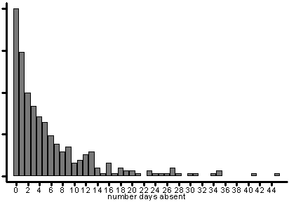
We will illustrate poisson regression using the lahigh data set. In particular, we would like to know whether there is a gender difference in days absent and the relation between language NCE test scores and days absent. Note that for gender, 0 is female and 1 is male. Here is a histogram of days absent.

use http://www.gseis.ucla.edu/courses/data/lahigh

summarize gender langnce daysabs

    Variable |     Obs        Mean   Std. Dev.       Min        Max
-------------+-----------------------------------------------------
      gender |     316    .4873418   .5006325          0          1
     langnce |     316    50.06379   17.93921   1.007114   98.99289
     daysabs |     316    5.810127   7.449003          0         45

summarize daysabs, detail

                         days absent
-------------------------------------------------------------
      Percentiles      Smallest
 1%            0              0
 5%            0              0
10%            0              0       Obs                 316
25%            1              0       Sum of Wgt.         316

50%            3                      Mean           5.810127
                        Largest       Std. Dev.      7.449003
75%            8             35
90%           14             35       Variance       55.48764
95%           23             41       Skewness       2.250587
99%           35             45       Kurtosis       8.949302


poisson daysabs gender langnce

Poisson regression                                Number of obs   =        316
                                                  LR chi2(2)      =     171.50
                                                  Prob > chi2     =     0.0000
Log likelihood = -1549.8567                       Pseudo R2       =     0.0524

------------------------------------------------------------------------------
     daysabs |      Coef.   Std. Err.      z    P>|z|     [95% Conf. Interval]
-------------+----------------------------------------------------------------
      gender |  -.4093528   .0482192    -8.49   0.000    -.5038606   -.3148449
     langnce |    -.01467   .0012934   -11.34   0.000    -.0172051   -.0121349
       _cons |   2.646977   .0697764    37.94   0.000     2.510217    2.783736
------------------------------------------------------------------------------

poisson, irr

Poisson regression                                Number of obs   =        316
                                                  LR chi2(2)      =     171.50
                                                  Prob > chi2     =     0.0000
Log likelihood = -1549.8567                       Pseudo R2       =     0.0524

------------------------------------------------------------------------------
     daysabs |        IRR   Std. Err.      z    P>|z|     [95% Conf. Interval]
-------------+----------------------------------------------------------------
      gender |   .6640799   .0320214    -8.49   0.000     .6041936    .7299021
     langnce |   .9854371   .0012746   -11.34   0.000      .982942    .9879384
------------------------------------------------------------------------------

listcoef  /* downloaded from Stata over the Internet */

poisson (N=316): Factor Change in Expected Count

 Observed SD: 7.4490028

------------------------------------------------------------------
 daysabs |      b         z     P>|z|    e^b    e^bStdX      SDofX
---------+--------------------------------------------------------
  gender |  -0.40935   -8.489   0.000   0.6641   0.8147     0.5006
 langnce |  -0.01467  -11.342   0.000   0.9854   0.7686    17.9392
------------------------------------------------------------------

listcoef, percent

poisson (N=316): Percentage Change in Expected Count

 Observed SD: 7.4490028

----------------------------------------------------------------------
     daysabs |      b         z     P>|z|      %      %StdX      SDofX
-------------+--------------------------------------------------------
      gender |  -0.40935   -8.489   0.000    -33.6    -18.5     0.5006
     langnce |  -0.01467  -11.342   0.000     -1.5    -23.1    17.9392
----------------------------------------------------------------------
InterpretationFrom the incidence rate ratios, being male decreases the expected number of days absent by a factor of .66, or equivalently, it decreases the expected number by 100*(.66-1)% = -33%. And, for each point increase in the language normal curve equivalence the expected number of days absent decreses by a factor of .98 (or 100*(.98-1)% = -2%) when the other variables are held constant.
The listcoef command also provides for standardized factor change. For a one standard deviation increase (approximately 18 points) in the language nce the expected number of days absent would decrease by a factor of .77 (100*(.77-1)% = -23%) with the other variables in the model held constant.
Another way of interpreting the model is to look at the marginal effects, also known as, partial change in the expected value.
mfx compute, at(mean)

Marginal effects after poisson
      y  = predicted number of events (predict)
         =  5.5458276
------------------------------------------------------------------------------
variable |      dy/dx    Std. Err.     z    P>|z|  [    95% C.I.   ]      X
---------+--------------------------------------------------------------------
  gender*|  -2.274269      .26514   -8.58   0.000  -2.79393  -1.7546   .487342
 langnce |  -.0813573      .00695  -11.70   0.000  -.094982 -.067733   50.0638
------------------------------------------------------------------------------
(*) dy/dx is for discrete change of dummy variable from 0 to 1

mfx compute, at(mean langnce=60)

Marginal effects after poisson
      y  = predicted number of events (predict)
         =     4.7936
------------------------------------------------------------------------------
variable |      dy/dx    Std. Err.     z    P>|z|  [    95% C.I.   ]      X
---------+--------------------------------------------------------------------
  gender*|   -1.96579      .22735   -8.65   0.000  -2.41139  -1.5202   .487342
 langnce |  -.0703221      .00515  -13.67   0.000  -.080408 -.060236   60.0000
------------------------------------------------------------------------------
(*) dy/dx is for discrete change of dummy variable from 0 to 1
Finally, we will look at the poisson goodness of fit. We should have looked at it earlier before
trying to interpret the model but we needed to take some time to discuss how one goes about
interpreting a poisson model.
poisgof

         Goodness-of-fit chi2  =  2238.317
         Prob > chi2(313)      =    0.0000
The large chi-square suggest that there is not a very good fit for the poisson regression
model. This could either be because the explanatory variables are not very good or
the poisson model is not appropriate. We saw earlier that the variance for daysabs was much
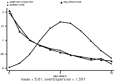
greater than the the mean. This suggest that there is overdispersion. We will use nbvargr to compare
the fit for poisson versus negabitive binomial models.
nbvargr daysabs  /* downloaded over the Internet */

Obtaining Parameter Estimates

(23 observations deleted)

  Negative Binomial Probabilities
  with mean = 5.810127 & overdispersion = 1.397268

        k     nbprob      nbcum
  1.    0  0.20559212  0.20559211
  2.    1  0.13100202  0.33659413
  3.    2  0.10005438  0.43664852
  4.    3  0.08063899  0.51728749
  5.    4  0.06669218  0.58397967
  6.    5  0.05600163  0.63998133
  7.    6  0.04749728  0.68747860
  8.    7  0.04057066  0.72804928
  9.    8  0.03483756  0.76288682
 10.    9  0.03003709  0.79292393
 11.   10  0.02598259  0.81890649

 Poisson Probabilities for lambda = 5.810127

        k      pprob       pcum
  1.    0  0.00299705  0.00299705
  2.    1  0.01741324  0.02041029
  3.    2  0.05058656  0.07099685
  4.    3  0.09797145  0.16896829
  5.    4  0.14230664  0.31127495
  6.    5  0.16536394  0.47663888
  7.    6  0.16013090  0.63676977
  8.    7  0.13291156  0.76968133
  9.    8  0.09652913  0.86621046
 10.    9  0.06231628  0.92852676
 11.   10  0.03620655  0.96473330

As we suspected, the poisson model did not do a good job of approximating daysabs.
The fact is overdispersion is very common in "real" data, the poisson distribution which works well
in theory does not perform all that well in practice.
The negative binomial model looks to be a much better fit.
Categorical Data Analysis Course
Phil Ender