
It wasn't that many years ago that when a researcher used regression, it was understood that the term referred to ordinary least squares (ols) regression. These days regression can refer to many different types analyses involving categorical and nonnormal response variables. In this class we will look into a number of these techniques.
In particular, we will cover models involving binary response variables; logit models, probit models and complementary loglog models. For categorical response variables with more than two levels, we will cover multinomial and ordered logit models. Regression with count variables will cover poisson and negative binomial regressions including the zero-inflated variations. All of these models will be related to one another using concepts from generalized linear models.
In addition, we will cover regression with censored and truncated data and introduce concepts for survival analysis.
I will be demonstrating the various procedures using the Stata statistics package. I have selected Stata because of the ease of distributing dataset and custom programs via the Internet. There are a number of statistical packages that have equivalent or nearly equivalent capabilities, including both SAS and SPSS. Additionally, several of the specialized packages, such as, HLM, Mplus and Splus, can analyze categorical and nonnormal data. Students may use any statistics package they are comfortable with.
In additional to the built-in Stata commands there is an excellent collection of programs written by J. Scott Long (University of Indiana) and Jeremy Freese (University of Wisconsin) that aid in the interpretation that we will use from time to time. Here are the Stata commands you can use to obtain these utilities via the Internet:
net from http://www.indiana.edu/~jslsoc/stata/
net install spostado
Some Terminology
A categorical variable is one which consists of a set of categories. Categorical variables can be dichotomous (two levels) or even more specifically binary (0/1). Binary variables can be ordered or unordered, it makes no difference in the analysis. When there are more than two categories the variables may have a natural ordering (ordinal variables) or no natural ordering (nominal variables). Nominal variables with more than two categories are analyzed using multinomial or polytomous models.
An interval variable has both order along with numerical distances between any two levels. In the measurement hierarchy, interval variables are the highest, ordinal variables are next followed by nominal variables. Statistical methods developed for one level can be used at a higher level but not at a lower one. For instance, methods developed for ordinal variables can be used with interval data (at the cost of discarding some of the information in the data) but could not be used with nominal variables.
Variables can be classified as continuous or discrete depending on the number of values they can take on. In practice, all variables are measured in a discrete manner due to limitations in measuring instruments. The real distinction between continuous and discrete is that continuous variables can take on many different values while discrete variables usually take on relatively few values.
Nominal variables are qualitative, that is, they differ in quality, not in quantity. Interval variables are clearly quantitative with different values differing in the amount of the variable. Ordinal variables fall somewhat indistinctly in between. They are often treated as qualitative and are analyzed using methods for nominal variables. At other times they treated as quantitative, almost on a par with interval variables. Some analysts consider these variables to be quasi-interval, that is, close enough to interval to allow interval methods to be used. Usually, quasi-interval variables take on more than five distinct values, although the cutoff point varies from researcher to researcher.
And finally, for the purposes of this class, the terms logistic regression, logit analysis and logit will be taken to mean the same techniques.
Conceptualizing Categorical Data Analysis
There are two primary approaches to conceptualizing categorical data analysis; 1) as a latent variable model or 2) as a nonlinear probability model.
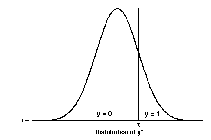
We will begin our discussion by considering the latent response model with a binary response variable. Consider an unobserved or latent variable y* that generates the observed values, the y's The observed values, the zeros and ones, are obtained by dividing the distribution of the latent variable into two regions. The larger values of y* are coded as y=1 while the smaller values are coded as y=0. A threshold or cutpoint, t, is used to divide the two portions of the y* distribution, as follows:


Historically, there has been a debate as to whether all categorical variables have an underlying, continuous latent variable or whether there are some variables that are naturally categorical. For those who don't wish to use the latent variable approach there are nonlinear probability models that lead to the same results.
Consider whether the following variables have an underlying latent variable:
Categorical Data Analysis Course
Phil Ender