Advanced Statistics
Regression Without Predictors
At first glance, it doesn't seem that studying regression without predictors
would be very useful. Certainly, we are not suggesting that using regression
without predictors is a major data analysis tool. We do think that it
is worthwhile to look at regression models without predictors to see what
they can tell us about the nature of the constant. Understanding the regression
constant in these simpler models will help us to understand both the
constant and the other regression coefficients in later more complex models.
The regression constant is also known as the intercept thus, regression
models without predictors are also known as intercept only models.
About the data
In this section we will use a sample of 200 observations taken from the
High School and Beyond (HSB) study (1986). We have selected the
variable write as our response or dependent variable. The values of write
represent standardized writing test scores from a test that was normalized
to have a mean equal to 50 and standard deviation of 10. The table below gives
the summary statistics for the variable write.
                                        -------------- Quantiles --------------
Variable       n     Mean     S.D.      Min      .25      Mdn      .75      Max
-------------------------------------------------------------------------------
   write     200    52.77     9.48    31.00    45.50    54.00    60.00    67.00
-------------------------------------------------------------------------------
OLS regression without predictors
Regression models are designed to estimate the expected mean of a response
(dependent) variable conditional on values of a set of predictor variables. An
ordinary least square regression equation with a single predictor variable can
be written as,
Yi = a + bXi + εi,
where Y is the response variable, X is a predictor variable and ε is the
residual or error. The coefficient b is the regression slope coefficient and a
is the constant or intercept. In the case where there are no predictors, this
equation reduces to,
Yi = a + εi.
In this unit, we are only interested in understanding and interpreting the
constant.
If we use the standard assumption that the residuals are normally distributed with mean zero
and variance σ2, i.e., εi ~ N(0,
σ2) then the expected value of the response variable is
E(Yi) = E(a + εi) =
a + E(εi) = a + 0 = mean(Y),
which is reduces to a = mean(Y) =  . That is, the constant
in the regression model is
a mean, in particular, in an intercept only model the constant is the mean
of the response variable.
Now, let's review how the sums of squares (SS) are partitioned into SS
for the regression model and SS for the residual.
SStotal = SSmodel + SSresidual

where Y is the response or observed variable,  is the mean and
  is the
predicted score. From now on we won't include all of the subscripts since it
will be understood that the summation is over one to n.
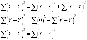
In an intercept only model the predicted score equals the mean, that is,
 =
=  . Therefore, we can replace
  with
with  in the sums of squares equation, leading to

This demonstrates that with an intercept only model there is only residual
variability; there is no variability due to the regression model because
there are no predictors. Now, let's run an intercept only model and see what
it looks like. The SPSS regression command does not allow for models without
predictora so we will use the closely related general linear model command, unianova.
 . That is, the constant
in the regression model is
a mean, in particular, in an intercept only model the constant is the mean
of the response variable.
 . That is, the constant
in the regression model is
a mean, in particular, in an intercept only model the constant is the mean
of the response variable.
 is the mean and
  is the
predicted score. From now on we won't include all of the subscripts since it
will be understood that the summation is over one to n.
 =
=  . Therefore, we can replace
  with
with  in the sums of squares equation, leading to